---
title: "12 · Coverage Depth Analysis"
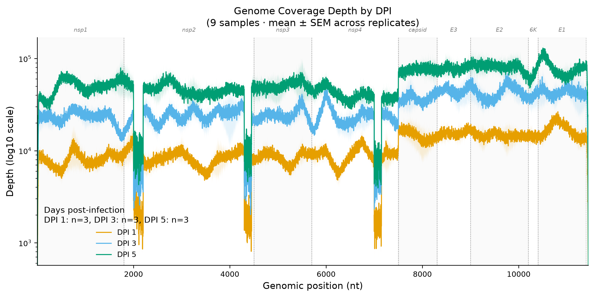
subtitle: "Per-position sequencing depth with gene annotations and DPI comparison"
description: |
Aggregates per-base sequencing depth across replicates grouped by days post-infection
(DPI). Produces a log-scale depth profile with gene boundary markers and SEM ribbons,
using the Okabe-Ito colorblind-safe palette.
categories: [genomics, virology, coverage, sequencing]
jupyter: python3
---
## Overview
| Item | Details |
|------|---------|
| **Input** | `coverage.csv` · `gene_coords.csv` · `manifest.csv` (generated by `data/simulate_data.py`) |
| **Key packages** | `pandas`, `numpy`, `matplotlib` |
| **Statistics** | Mean depth ± SEM per position (aggregated across replicates) |
| **Output** | Coverage depth profile (PNG + SVG) with gene annotations · aggregated summary CSV |
| **Download** | [template.qmd](template.qmd) |
[← Gallery](../../index.html){.btn .btn-outline-secondary}
[Download .qmd](template.qmd){.btn .btn-primary}
---
## User Configuration
```{python}
#| label: user-config
# ── USER CONFIGURATION ────────────────────────────────────────────────────────

# Data directory (relative to this notebook)
DATA_DIR = "data"

# Output directory for figures and summary tables
OUTPUT_DIR = "outputs"

# Okabe-Ito colorblind-safe palette (mapped to DPI values in display order).
# Any DPI present in the data but absent here falls back to the palette cycle below.
DPI_COLORS = {
    1: "#E69F00",   # orange
    3: "#56B4E9",   # sky blue
    5: "#009E73",   # bluish green
}

# Fallback palette for DPI values not listed in DPI_COLORS
OKABE_ITO_CYCLE = ["#E69F00", "#56B4E9", "#009E73", "#F0E442",
                   "#0072B2", "#D55E00", "#CC79A7", "#000000"]

# Display order for DPI groups. None = derive (ascending) from the data, which is
# what you want unless you need a specific non-numeric ordering.
DPI_ORDER = None

# Figure dimensions (inches)
FIG_WIDTH  = 12
FIG_HEIGHT = 5

# Figure DPI for PNG raster output
FIG_DPI = 300

# Log scale toggle (True = log10 y-axis)
LOG_SCALE = True

# ─────────────────────────────────────────────────────────────────────────────
```
## Setup
```{python}
#| label: setup
import os
import warnings

import pandas as pd
import matplotlib.pyplot as plt

# Narrow suppression only: matplotlib emits this for any non-positive value on a
# log axis. Zero-depth positions are reported explicitly further down instead.
warnings.filterwarnings("ignore", category=UserWarning,
                        message="Data has no positive values")

os.makedirs(OUTPUT_DIR, exist_ok=True)

# ── Publication‑ready matplotlib style (white bg, no grid, black spines) ─────

# Reproducible SVG output: matplotlib stamps a wall-clock date and randomly
# generated element IDs into every SVG, so re-rendering an unchanged figure
# produced a large but meaningless git diff. A fixed salt and a fixed
# SOURCE_DATE_EPOCH make repeat renders byte-identical.
os.environ.setdefault("SOURCE_DATE_EPOCH", "1735689600")   # 2025-01-01 UTC
plt.rcParams["svg.hashsalt"] = "lab-bioinfo-templates"

plt.rcParams.update({
    "axes.facecolor":       "white",
    "figure.facecolor":     "white",
    "savefig.facecolor":    "white",
    "axes.grid":            False,
    "axes.edgecolor":       "black",
    "axes.linewidth":       0.8,
    "xtick.color":          "black",
    "ytick.color":          "black",
    "axes.spines.top":      False,
    "axes.spines.right":    False,
    "font.family":          "sans-serif",
    "font.sans-serif":      ["Arial", "DejaVu Sans"],
    "font.size":            10,
    "axes.titlesize":       12,
    "axes.labelsize":       11,
    "xtick.labelsize":      9,
    "ytick.labelsize":      9,
    "legend.fontsize":      9,
    "legend.frameon":       False,
    "figure.dpi":           100,
    "savefig.dpi":          300,
    "savefig.bbox":         "tight",
})

print(f"Output will be saved to: {os.path.abspath(OUTPUT_DIR)}")
```
## Load Data
```{python}
#| label: load-data
def require_columns(df, required, name):
    """Fail loudly if an input table is missing a column the analysis depends on."""
    missing = set(required) - set(df.columns)
    if missing:
        raise ValueError(
            f"{name} is missing required column(s): {sorted(missing)}. "
            f"Found: {list(df.columns)}"
        )

cov      = pd.read_csv(os.path.join(DATA_DIR, "coverage.csv"))
genes    = pd.read_csv(os.path.join(DATA_DIR, "gene_coords.csv"))
manifest = pd.read_csv(os.path.join(DATA_DIR, "manifest.csv"))

require_columns(cov, ["Position", "Depth", "sample_id", "dpi"], "coverage.csv")
require_columns(genes, ["gene", "start", "end"], "gene_coords.csv")
require_columns(manifest, ["sample_id", "dpi", "replicate"], "manifest.csv")

# Display order for DPI groups, plus a colour for every one of them.
dpi_order = list(DPI_ORDER) if DPI_ORDER else sorted(cov["dpi"].dropna().unique())
unconfigured = [d for d in sorted(cov["dpi"].dropna().unique()) if d not in dpi_order]
if unconfigured:
    raise ValueError(
        f"DPI_ORDER does not list every DPI present in coverage.csv: {unconfigured} "
        f"would be dropped from the figure. Configured: {dpi_order}. "
        f"Set DPI_ORDER = None to derive it from the data."
    )

dpi_colors = {
    d: DPI_COLORS.get(d, OKABE_ITO_CYCLE[i % len(OKABE_ITO_CYCLE)])
    for i, d in enumerate(dpi_order)
}

print(f"Coverage:  {len(cov):,} rows · {cov['sample_id'].nunique()} samples")
print(f"Genes:     {len(genes)} annotated features")
print(f"Manifest:  {len(manifest)} samples across {manifest['dpi'].nunique()} DPI groups")
print(f"DPI order: {dpi_order}")

cov.head(5)
```
```{python}
#| label: preview-genes
genes
```
## Aggregate Depth by DPI
```{python}
#| label: aggregate-depth
agg = (
    cov.groupby(["dpi", "Position"])["Depth"]
       .agg(["mean", "sem", "count"])
       .reset_index()
)

print(f"Aggregated depth table: {len(agg)} rows (position × DPI)")
agg.head(8)
```
```{python}
#| label: check-dpi-groups
for dpi_val in dpi_order:
    sub = agg[agg["dpi"] == dpi_val]
    n_reps = manifest[manifest["dpi"] == dpi_val]["replicate"].nunique()
    per_pos = sorted(sub["count"].unique())
    print(
        f"  DPI {dpi_val}: {n_reps} replicates, "
        f"mean depth = {sub['mean'].mean():.0f} ± {sub['sem'].mean():.0f} SEM "
        f"({per_pos} replicate(s) per position)"
    )
```
## Coverage Depth Plot
```{python}
#| label: coverage-plot
#| fig-width: 12
#| fig-height: 5
fig, ax = plt.subplots(figsize=(FIG_WIDTH, FIG_HEIGHT))

# ── Gene boundary vertical lines and labels ───────────────────────────────────

for _, gene in genes.iterrows():
    ax.axvline(gene["start"],  color="grey", linestyle="--", linewidth=0.5, alpha=0.5)
    ax.axvline(gene["end"],    color="grey", linestyle="--", linewidth=0.5, alpha=0.5)
    midpoint = (gene["start"] + gene["end"]) / 2
    ax.annotate(
        gene["gene"],
        xy=(midpoint, 1.02),
        xycoords=("data", "axes fraction"),
        ha="center",
        va="bottom",
        fontsize=7,
        fontstyle="italic",
        color="grey",
    )

# ── Alternating gene background shading ───────────────────────────────────────

for i, (_, gene) in enumerate(genes.iterrows()):
    if i % 2 == 0:
        ax.axvspan(gene["start"], gene["end"], alpha=0.04, color="grey", zorder=0)

# ── Depth curves with SEM ribbons ─────────────────────────────────────────────

genome_start = agg["Position"].min()
genome_end   = agg["Position"].max()

for dpi_val in dpi_order:
    sub = agg[agg["dpi"] == dpi_val].sort_values("Position")
    color = dpi_colors[dpi_val]
    ax.plot(
        sub["Position"],
        sub["mean"],
        color=color,
        linewidth=1.2,
        label=f"DPI {dpi_val}",
        zorder=2,
    )
    ax.fill_between(
        sub["Position"],
        sub["mean"] - sub["sem"],
        sub["mean"] + sub["sem"],
        color=color,
        alpha=0.15,
        linewidth=0,
        zorder=1,
    )

# ── Axes and labels ───────────────────────────────────────────────────────────

ax.set_xlim(genome_start, genome_end)
ax.set_xlabel("Genomic position (nt)")

if LOG_SCALE:
    ax.set_yscale("log")
    # Plain "log10": the ₁₀ subscript glyph is missing from Arial and renders as
    # tofu boxes on the published figure.
    ax.set_ylabel("Depth (log10 scale)")
    # Bound the log axis by the data, not by a magic floor: a hardcoded lower
    # limit silently pushes low-depth positions off the bottom of the chart.
    positive = agg.loc[agg["mean"] > 0, "mean"]
    n_zero = int((agg["mean"] <= 0).sum())
    if n_zero:
        print(f"Note: {n_zero} position×DPI mean(s) are 0 and cannot be shown "
              f"on a log axis — switch LOG_SCALE to False to see them.")
    # The terminal tapers drive depth toward zero at both genome ends. Bounding the
    # axis by the outright minimum would hand half the plot to those few bases, so
    # bound by a low percentile and let the tapers run off the bottom.
    floor = max(positive.quantile(0.001) * 0.5, positive.min() * 0.7)
    ax.set_ylim(floor, agg["mean"].max() * 1.3)
else:
    ax.set_ylabel("Sequencing depth")
    ax.set_ylim(0, agg["mean"].max() * 1.15)

ax.set_title(
    "Genome Coverage Depth by DPI\n"
    f"({len(manifest['sample_id'].unique())} samples · mean ± SEM across replicates)",
    fontsize=12,
    pad=14,
)

n_per_dpi = manifest.groupby("dpi")["sample_id"].nunique()
legend_title = "Days post-infection\n" + ", ".join(
    f"DPI {d}: n={int(n_per_dpi.get(d, 0))}" for d in dpi_order
)

ax.legend(
    title=legend_title,
    loc="lower left",   # upper right sits on top of the depth curves
    frameon=False,
)

# ── Save ──────────────────────────────────────────────────────────────────────

for fmt in ["png", "svg"]:
    out_path = os.path.join(OUTPUT_DIR, f"coverage_depth.{fmt}")
    fig.savefig(out_path, format=fmt, dpi=FIG_DPI)
    print(f"Saved: {os.path.abspath(out_path)}")

plt.show()
```
## Summary Export
```{python}
#| label: summary-export
agg.to_csv(os.path.join(OUTPUT_DIR, "coverage_depth_summary.csv"), index=False)
print(f"Saved: {os.path.join(OUTPUT_DIR, 'coverage_depth_summary.csv')}")

# Per-DPI genome-wide summary
per_dpi = (
    agg.groupby("dpi")
       .agg(
           mean_depth=("mean", "mean"),
           median_depth=("mean", "median"),
           min_depth=("mean", "min"),
           max_depth=("mean", "max"),
           mean_sem=("sem", "mean"),
       )
       .round(1)
)

per_dpi
```
---
*Analysis complete.* Depth profile saved to `` `{python} OUTPUT_DIR + "/"` ``.