06 · GO Enrichment Analysis

Gene Ontology, KEGG pathway enrichment, and multi-comparison bubble plots

genomics

KEGG

enrichment

Performs GO (Biological Process) and KEGG pathway enrichment analysis across one or more DESeq2 comparisons. Produces publication-quality bubble plots for user-defined gene sets, enrichment dot plots, and wide-format CSV exports for GraphPad/Prism.

Overview

Item	Details
Input	CSV with columns: `Gene`, `Comparison`, `log2FoldChange`, `padj`
Key packages	`clusterProfiler`, `enrichplot`, `ggplot2`, `viridis`, `patchwork`
Statistics	GO enrichment (BP/MF/CC) · KEGG pathway enrichment · BH-FDR
Output	Bubble plots (SVG) · GO/KEGG dot plots · Enrichment CSVs
Download	template.Rmd

Tip

When to use this template: You have DESeq2 results from one or more comparisons and want to visualize the expression of curated gene sets as bubble plots, and run GO/KEGG enrichment on significant DEGs.

Note

Bubble plot style: theme_bw() with blank panel grids · viridis plasma color scale · italic y-axis gene labels · legend on the left.

Back to Gallery Open Template File

Code

## ── USER CONFIGURATION ──────────────────────────────────────────────────────
#
# DEG_FILE: CSV file with differential expression results.
#   Required columns: Gene, Comparison, log2FoldChange, padj
#   One row per gene per comparison.
#
DEG_FILE <- "data/deg_results.csv"

# ORG_DB: Bioconductor annotation package for your species.
#   Must have an entry in KEGG_ORGANISM_CODES below, otherwise the KEGG
#   section stops with an error rather than silently querying another species.
ORG_DB   <- "org.Mm.eg.db"
SPECIES  <- "Mus musculus"   # used in plot subtitles

# KEGG_ORGANISM_CODES: OrgDb package -> KEGG three-letter organism code.
#   Add your species here if it is missing (see https://rest.kegg.jp/list/organism).
KEGG_ORGANISM_CODES <- c(
  "org.Hs.eg.db" = "hsa",   # human
  "org.Mm.eg.db" = "mmu",   # mouse
  "org.Rn.eg.db" = "rno",   # rat
  "org.Dm.eg.db" = "dme",   # fruit fly
  "org.Dr.eg.db" = "dre",   # zebrafish
  "org.Ce.eg.db" = "cel",   # C. elegans
  "org.Sc.sgd.db" = "sce",  # budding yeast
  "org.Gg.eg.db" = "gga",   # chicken
  "org.Bt.eg.db" = "bta",   # cow
  "org.Ss.eg.db" = "ssc",   # pig
  "org.Cf.eg.db" = "cfa",   # dog
  "org.Mmu.eg.db" = "mcc",  # rhesus macaque
  "org.At.tair.db" = "ath"  # Arabidopsis
)

# FDR_THRESHOLD: Significance threshold for identifying DEGs.
FDR_THRESHOLD   <- 0.05

# LFC_THRESHOLD: |log2FoldChange| cutoff for bubble plots and enrichment.
LFC_THRESHOLD   <- 1.5

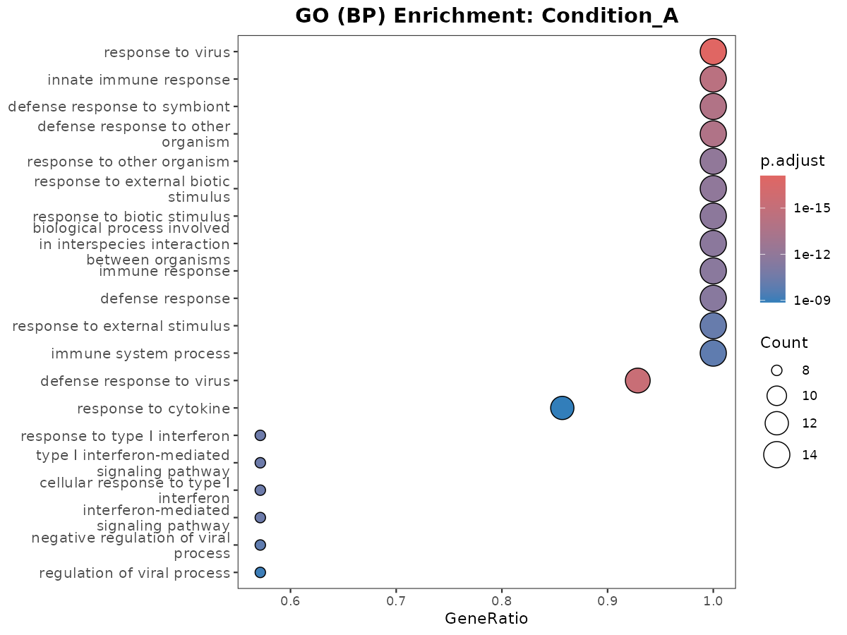
# ENRICHMENT_FDR: FDR cutoff for reporting enriched terms.
ENRICHMENT_FDR  <- 0.05

# MIN_GENE_SET / MAX_GENE_SET: Gene set size limits for enrichment.
MIN_GENE_SET    <- 10
MAX_GENE_SET    <- 500

# COMPARISONS_ORDER: Factor order for the x-axis of bubble plots.
#   Must match the "Comparison" values in DEG_FILE.
#   NULL = use alphabetical order.
COMPARISONS_ORDER <- NULL   # e.g., c("Condition_A", "Condition_B", "Condition_C")

# COMPARISON_LABELS: Human-readable x-axis labels (same length as COMPARISONS_ORDER).
#   NULL = use raw comparison names.
COMPARISON_LABELS <- NULL   # e.g., c("Group A vs Ctrl", "Group B vs Ctrl", ...)

# GENE_SETS: Named list of character vectors for bubble-plot gene sets.
#   Each element is one panel / pathway.
#   Replace these with your gene lists of interest.
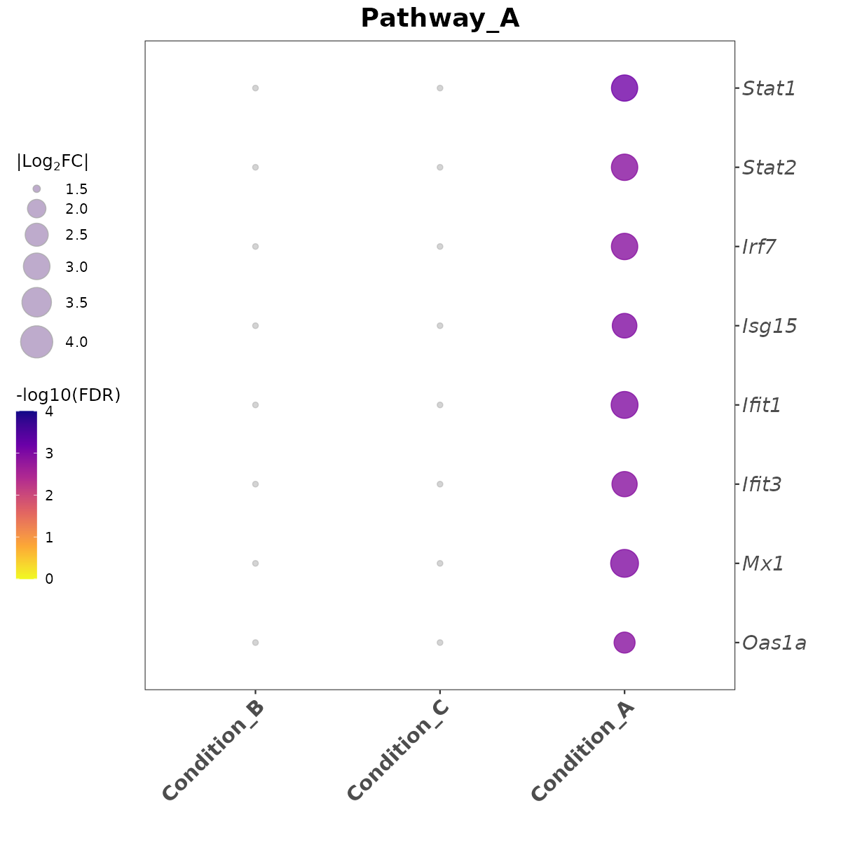
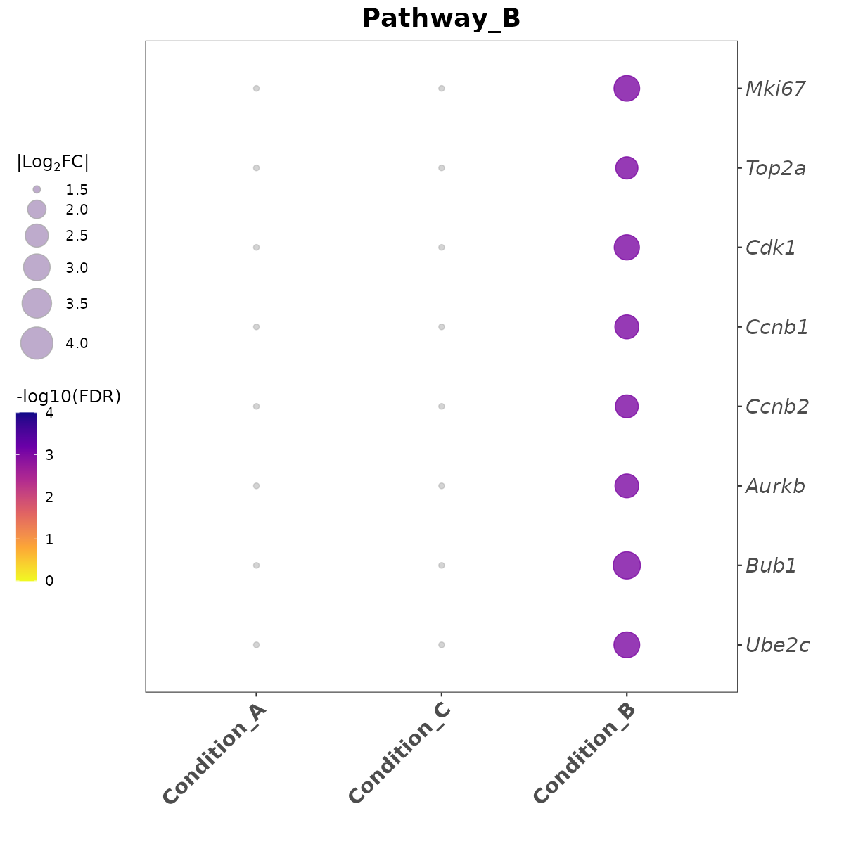
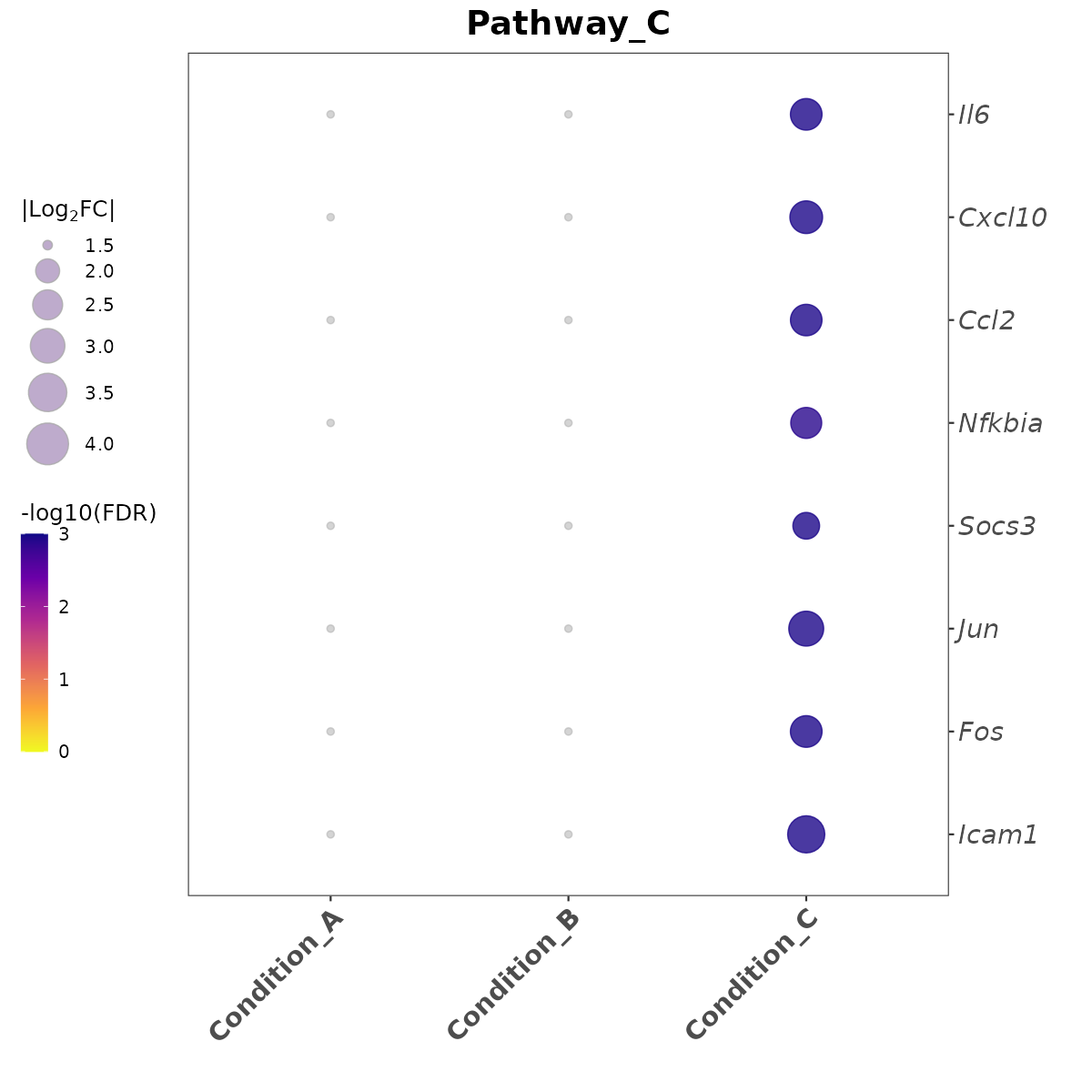
GENE_SETS <- list(
  Pathway_A = c("Stat1", "Stat2", "Irf7", "Isg15", "Ifit1",
                "Ifit3", "Mx1", "Oas1a"),
  Pathway_B = c("Mki67", "Top2a", "Cdk1", "Ccnb1", "Ccnb2",
                "Aurkb", "Bub1", "Ube2c"),
  Pathway_C = c("Il6", "Cxcl10", "Ccl2", "Nfkbia", "Socs3",
                "Jun", "Fos", "Icam1")
)

# OUTPUT_DIR: Where to save plots and data exports.
OUTPUT_DIR <- "Plots"

## ────────────────────────────────────────────────────────────────────────────

Setup

Code

# tidyverse attaches ggplot2, dplyr, readr, stringr, tidyr and purrr, so
# loading those individually as well only adds noise and masking messages.
library(tidyverse)
library(clusterProfiler)
library(enrichplot)
library(RColorBrewer)
library(viridis)
library(svglite)
library(patchwork)
library(scales)

org_db <- get(ORG_DB, envir = asNamespace(ORG_DB))

# Resolve the KEGG organism code up front, so an unsupported OrgDb fails here
# with a clear message instead of running enrichment against the wrong species.
if (!ORG_DB %in% names(KEGG_ORGANISM_CODES)) {
  stop("No KEGG organism code configured for ORG_DB = '", ORG_DB, "'.\n",
       "  Add it to KEGG_ORGANISM_CODES in the user-configuration block.\n",
       "  Currently configured: ",
       paste(names(KEGG_ORGANISM_CODES), collapse = ", "))
}
KEGG_ORGANISM <- unname(KEGG_ORGANISM_CODES[[ORG_DB]])
message("ORG_DB = ", ORG_DB, " -> KEGG organism = ", KEGG_ORGANISM)

# Filenames must never contain characters that are illegal or awkward on a
# filesystem or in a URL. Comparison labels are user-supplied free text
# (COMPARISON_LABELS explicitly supports things like "Group A vs Ctrl"), so
# every path AND every <img src> below is built from the sanitized form.
sanitize_filename <- function(x) {
  gsub("^_+|_+$", "", gsub("[^A-Za-z0-9_.-]+", "_", as.character(x)))
}

dir.create(file.path(OUTPUT_DIR, "Bubble_Plots"),    recursive = TRUE, showWarnings = FALSE)
dir.create(file.path(OUTPUT_DIR, "Enrichment"),      recursive = TRUE, showWarnings = FALSE)
dir.create(file.path(OUTPUT_DIR, "Pathway_Heatmaps"),recursive = TRUE, showWarnings = FALSE)

Load Data

Code

deg_all <- read_csv(DEG_FILE, show_col_types = FALSE)

# Set factor levels for comparisons
if (!is.null(COMPARISONS_ORDER)) {
  deg_all <- deg_all %>%
    mutate(Comparison = factor(Comparison, levels = COMPARISONS_ORDER,
                               labels = if (!is.null(COMPARISON_LABELS)) COMPARISON_LABELS
                                        else COMPARISONS_ORDER))
} else {
  deg_all <- deg_all %>% mutate(Comparison = factor(Comparison))
}

# Mark significant genes.
# padj == 0 (underflow in the upstream DE test) must not become NA: that would
# render the MOST significant genes in the plot's na.value grey. Floor at the
# smallest representable double instead, as template 07 does.
deg_all <- deg_all %>%
  mutate(
    padj_plot   = pmax(dplyr::coalesce(padj, 1), .Machine$double.xmin),
    log_padj    = -log10(padj_plot),
    significant = !is.na(padj) & padj < FDR_THRESHOLD & abs(log2FoldChange) >= LFC_THRESHOLD
  )

deg_summary <- deg_all %>%
  group_by(Comparison) %>%
  summarise(
    `Total Genes`   = n_distinct(Gene),
    `Significant DEGs` = sum(significant, na.rm = TRUE),
    `Upregulated`   = sum(significant & log2FoldChange >= LFC_THRESHOLD, na.rm = TRUE),
    `Downregulated` = sum(significant & log2FoldChange <= -LFC_THRESHOLD, na.rm = TRUE),
    .groups = "drop"
  )

deg_summary %>%
  knitr::kable(
    caption   = sprintf(
      "Differential Expression Summary per Comparison (|Log2FC| >= %s & FDR < %s)",
      format(LFC_THRESHOLD), format(FDR_THRESHOLD)),
    col.names = c("Comparison", "Total Genes", "Significant DEGs", "Upregulated", "Downregulated"),
    format.args = list(big.mark = ",")
  )

Differential Expression Summary per Comparison (|Log2FC| >= 1.5 & FDR < 0.05)
Comparison	Total Genes	Significant DEGs	Upregulated	Downregulated
Condition_A	2,045	15	15	0
Condition_B	2,045	15	0	15
Condition_C	2,045	15	15	0

Bubble Plots (Gene Set Visualization)

Pathway_A

Pathway_B

Pathway_C

Data Export (Wide Format)

Code

dir.create(file.path(OUTPUT_DIR, "Pathway_Heatmaps"), showWarnings = FALSE, recursive = TRUE)

for (nm in names(GENE_SETS)) {
  safe_name <- bubble_files[[nm]]

  wide_lfc <- deg_all %>%
    filter(Gene %in% GENE_SETS[[nm]]) %>%
    mutate(lfc_masked = ifelse(significant, log2FoldChange, 0)) %>%
    select(Gene, Comparison, lfc_masked) %>%
    tidyr::pivot_wider(names_from = Comparison, values_from = lfc_masked, values_fill = 0)

  write_csv(wide_lfc, file.path(OUTPUT_DIR, "Pathway_Heatmaps",
                                 paste0("GraphPad_", safe_name, ".csv")))
}
message("Exported wide-format CSVs to ", file.path(OUTPUT_DIR, "Pathway_Heatmaps"))

Exported wide-format CSVs to Plots/Pathway_Heatmaps

GO Enrichment Analysis

Code

# ── Background gene set (universe) ────────────────────────────────────────────
# Without `universe=`, clusterProfiler uses every annotated gene in the OrgDb
# (tens of thousands) as the background for a few hundred tested genes. That is
# the classic GO error: it systematically inflates every enrichment p-value.
# The correct background is the set of genes that were actually TESTED —
# i.e. everything present in DEG_FILE, significant or not.
universe_ids <- tryCatch(
  bitr(unique(deg_all$Gene), fromType = "SYMBOL", toType = "ENTREZID", OrgDb = org_db),
  error = function(e) NULL
)

Warning in bitr(unique(deg_all$Gene), fromType = "SYMBOL", toType = "ENTREZID",
: 0.05% of input gene IDs are fail to map...

Code

if (is.null(universe_ids) || nrow(universe_ids) == 0) {
  stop("Could not map any gene symbol in DEG_FILE to an ENTREZID via ", ORG_DB,
       " - check that ORG_DB matches the species of your DEG table.")
}
GENE_UNIVERSE <- unique(universe_ids$ENTREZID)

cat(sprintf("Background universe: %d of %d tested symbols mapped to Entrez IDs.\n",
            length(GENE_UNIVERSE), n_distinct(deg_all$Gene)))

Background universe: 2044 of 2045 tested symbols mapped to Entrez IDs.

Condition_A

Condition_B

Condition_C

KEGG Pathway Enrichment

Condition_A

Condition_B

Condition_C