05 · Phylo-Geographic Analysis

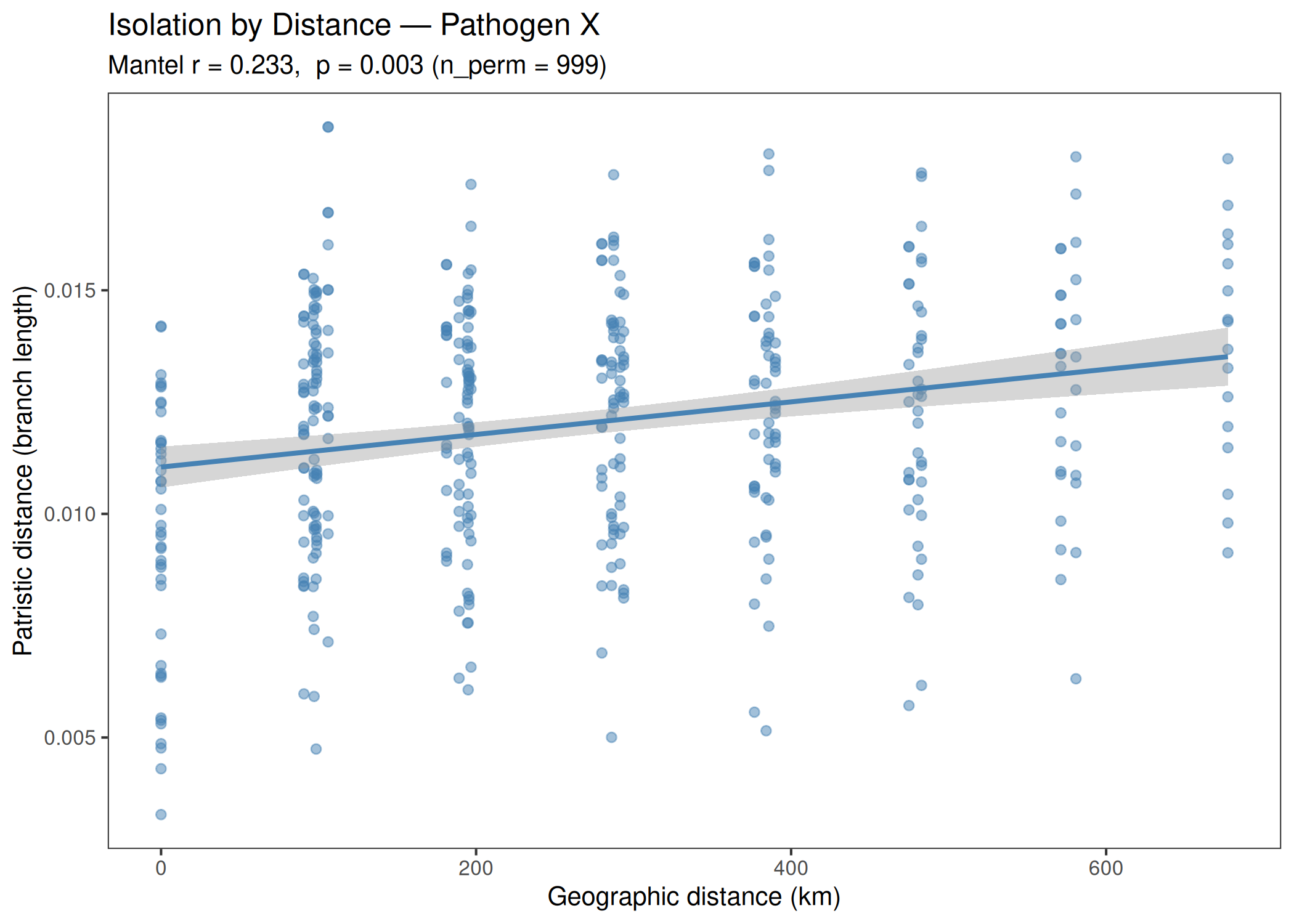
Isolation by Distance (Mantel Test), Scatter Pie Map, and Mantel Correlogram

phylogenetics

geographic

mantel

virology

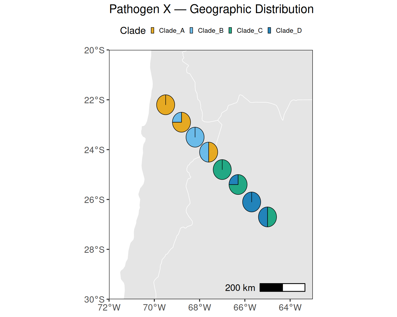
Performs isolation-by-distance analysis using Mantel tests on patristic distances from a phylogenetic tree and geographic (Haversine) distances. Produces a scatter pie map showing clade composition per sampling location and a Mantel correlogram.

Overview

Item	Details
Input	Aligned FASTA (S segment required, M optional) · Newick tree · coordinates CSV · metadata CSV
Key packages	`ape`, `vegan`, `geosphere`, `scatterpie`, `sf`, `rnaturalearth`, `ggspatial`
Statistics	Mantel test (Pearson) · patristic distances · Haversine geographic distances
Output	Isolation-by-distance plot · scatter pie map · Mantel correlogram · TIFF + SVG
Download	template.Rmd

Tip

When to use this template: You have a phylogenetic tree and sampling coordinates for a pathogen, and want to test whether genetic distance correlates with geographic distance (isolation by distance) and visualize the geographic distribution of clades.

Note

Clade colors: Default palette uses Okabe-Ito colorblind-safe colors. Update CLADE_COLORS in the USER CONFIGURATION block to match your clade assignments. The scatter pie radius (radius column in pie_data) is in degrees — adjust mutate(radius = 0.4) to scale pies appropriately for your map extent.

Back to Gallery Open Template File

Code

## ── USER CONFIGURATION ──────────────────────────────────────────────────────
#
# Input files:
S_FASTA    <- "data/S_aligned.fasta"   # Aligned S-segment FASTA
M_FASTA    <- "data/M_aligned.fasta"   # Aligned M-segment FASTA  (optional)
TREEFILE   <- "data/S_tree.nwk"        # Newick tree from IQ-TREE or similar
COORDS_FILE<- "data/coordinates.csv"   # Columns: SampleID, Longitude, Latitude
METADATA_FILE <- "data/metadata.csv"   # Columns: SampleID, Clade (+ optional extras)

# Column names in COORDS_FILE and METADATA_FILE that link to FASTA tip labels.
SAMPLE_COL <- "SampleID"

# Columns in METADATA_FILE used for clade coloring.
CLADE_COL  <- "Clade"

# CLADE_COLORS: Named color vector (Okabe-Ito palette).
#   Names must match the unique values in METADATA_FILE[[CLADE_COL]].
CLADE_COLORS <- c(
  "Clade_A" = "#E69F00",   # Orange
  "Clade_B" = "#56B4E9",   # Sky blue
  "Clade_C" = "#009E73",   # Bluish green
  "Clade_D" = "#0072B2"    # Blue
)

# PATHOGEN_NAME: Used in plot titles and axis labels.
PATHOGEN_NAME <- "Pathogen X"

# Mantel test: number of permutations (increase to 99999 for publication).
MANTEL_NPERM <- 999

# Map extent (degrees): lon/lat range around your sampling area.
MAP_LON <- c(-72, -63)
MAP_LAT <- c(-30, -20)

# OUTPUT_DIR: Where to save plots.
OUTPUT_DIR <- "Plots"

## ────────────────────────────────────────────────────────────────────────────

Setup

Code

library(ape)
library(vegan)
library(geosphere)
library(Biostrings)
library(tidyverse)
library(sf)
library(rnaturalearth)
library(rnaturalearthdata)
library(ggspatial)
library(scatterpie)
library(svglite)
library(patchwork)
library(ragg)

dir.create(file.path(OUTPUT_DIR, "Maps"),    recursive = TRUE, showWarnings = FALSE)
dir.create(file.path(OUTPUT_DIR, "Mantel"),  recursive = TRUE, showWarnings = FALSE)

Load Data

Code

# FASTA sequences
seqs_S <- readDNAStringSet(S_FASTA)

# Phylogenetic tree
tree_S <- read.tree(TREEFILE)

# Metadata & coordinates
coords   <- read_csv(COORDS_FILE, show_col_types = FALSE)
metadata <- read_csv(METADATA_FILE, show_col_types = FALSE)

# Combine
sample_data <- coords %>%
  left_join(metadata, by = SAMPLE_COL) %>%
  filter(!is.na(Longitude), !is.na(Latitude))

cat("Sequences loaded:", length(seqs_S), "\n")

Sequences loaded: 30

Code

cat("Samples with coordinates:", nrow(sample_data), "\n")

Samples with coordinates: 30

Code

print(head(sample_data))

# A tibble: 6 × 6
  SampleID Longitude Latitude Clade    Year Host    
  <chr>        <dbl>    <dbl> <chr>   <dbl> <chr>   
1 Sample_1     -69.5    -22.2 Clade_A  2019 Rodent_A
2 Sample_2     -69.5    -22.2 Clade_A  2018 Rodent_B
3 Sample_3     -69.5    -22.2 Clade_A  2015 Rodent_B
4 Sample_4     -69.5    -22.2 Clade_A  2020 Rodent_A
5 Sample_5     -68.8    -22.9 Clade_A  2021 Rodent_A
6 Sample_6     -68.8    -22.9 Clade_A  2022 Rodent_A

Replicate Agreement / Sequence Alignment QC

Code

seq_widths <- width(seqs_S)
cat(sprintf("S alignment: %d sequences, length %d–%d bp\n",
            length(seq_widths), min(seq_widths), max(seq_widths)))

S alignment: 30 sequences, length 1200–1200 bp

Code

# Count ambiguous bases per sequence
ambig_counts <- sapply(as.character(seqs_S), function(s)
  sum(strsplit(s, "")[[1]] %in% c("N","R","Y","S","W","K","M","B","D","H","V")))

data.frame(
  sequence    = names(seqs_S),
  length      = seq_widths,
  ambig_bases = ambig_counts
) %>% arrange(desc(ambig_bases))

           sequence length ambig_bases
Sample_1   Sample_1   1200           0
Sample_2   Sample_2   1200           0
Sample_3   Sample_3   1200           0
Sample_4   Sample_4   1200           0
Sample_5   Sample_5   1200           0
Sample_6   Sample_6   1200           0
Sample_7   Sample_7   1200           0
Sample_8   Sample_8   1200           0
Sample_9   Sample_9   1200           0
Sample_10 Sample_10   1200           0
Sample_11 Sample_11   1200           0
Sample_12 Sample_12   1200           0
Sample_13 Sample_13   1200           0
Sample_14 Sample_14   1200           0
Sample_15 Sample_15   1200           0
Sample_16 Sample_16   1200           0
Sample_17 Sample_17   1200           0
Sample_18 Sample_18   1200           0
Sample_19 Sample_19   1200           0
Sample_20 Sample_20   1200           0
Sample_21 Sample_21   1200           0
Sample_22 Sample_22   1200           0
Sample_23 Sample_23   1200           0
Sample_24 Sample_24   1200           0
Sample_25 Sample_25   1200           0
Sample_26 Sample_26   1200           0
Sample_27 Sample_27   1200           0
Sample_28 Sample_28   1200           0
Sample_29 Sample_29   1200           0
Sample_30 Sample_30   1200           0

Isolation by Distance (Mantel Test)

Code

# ── 1. Patristic distance matrix from tree ─────────────────────────────────────
patristic_mat <- cophenetic.phylo(tree_S)

# ── 2. Geographic distance matrix (great-circle, km) ──────────────────────────
# Match order to tree tips
tip_ids <- tree_S$tip.label

# Extract SampleID from tip label (adjust regex to your naming convention)
tip_sample_ids <- str_extract(tip_ids, "Sample_[0-9]+")

coords_ordered <- sample_data %>%
  filter(get(SAMPLE_COL) %in% tip_sample_ids) %>%
  slice(match(tip_sample_ids, get(SAMPLE_COL)))

geo_mat <- distm(
  cbind(coords_ordered$Longitude, coords_ordered$Latitude),
  fun = distHaversine
) / 1000   # → km

rownames(geo_mat) <- colnames(geo_mat) <- coords_ordered[[SAMPLE_COL]]

# ── 3. Mantel test ─────────────────────────────────────────────────────────────
# Subset to shared taxa
shared  <- intersect(rownames(patristic_mat), rownames(geo_mat))
pat_sub <- patristic_mat[shared, shared]
geo_sub <- geo_mat[shared, shared]

mantel_result <- mantel(pat_sub, geo_sub,
                         method  = "pearson",
                         permutations = MANTEL_NPERM)
print(mantel_result)


Mantel statistic based on Pearson's product-moment correlation 

Call:
mantel(xdis = pat_sub, ydis = geo_sub, method = "pearson", permutations = MANTEL_NPERM) 

Mantel statistic r: 0.233 
      Significance: 0.003 

Upper quantiles of permutations (null model):
  90%   95% 97.5%   99% 
0.110 0.135 0.158 0.175 
Permutation: free
Number of permutations: 999

Code

# ── 4. Scatter plot ────────────────────────────────────────────────────────────
ibd_df <- data.frame(
  geographic  = as.vector(geo_sub[lower.tri(geo_sub)]),
  phylogenetic = as.vector(pat_sub[lower.tri(pat_sub)])
)

p_ibd <- ggplot(ibd_df, aes(x = geographic, y = phylogenetic)) +
  geom_point(alpha = 0.5, size = 1.5, color = "steelblue") +
  geom_smooth(method = "lm", color = "steelblue", se = TRUE) +
  labs(
    title = paste("Isolation by Distance —", PATHOGEN_NAME),
    subtitle = sprintf("Mantel r = %.3f,  p = %.3f (n_perm = %d)",
                       mantel_result$statistic, mantel_result$signif, MANTEL_NPERM),
    x = "Geographic distance (km)",
    y = "Patristic distance (branch length)"
  ) +
  theme_bw(base_size = 10, base_family = "sans") +
  theme(
    panel.grid.major = element_blank(),
    panel.grid.minor = element_blank()
  )

ggsave(file.path(OUTPUT_DIR, "Mantel", "isolation_by_distance.tiff"),
       plot = p_ibd, width = 3, height = 3, dpi = 300,
       device = "tiff", compression = "lzw")
print(p_ibd)

Scatter Pie Map

Code

# ── Summarize clade composition per location ───────────────────────────────────
# (when multiple samples share a location, show their clade proportions as a pie)
pie_data <- sample_data %>%
  group_by(Longitude, Latitude, !!sym(CLADE_COL)) %>%
  summarise(n = n(), .groups = "drop") %>%
  tidyr::pivot_wider(names_from = all_of(CLADE_COL), values_from = n, values_fill = 0) %>%
  mutate(radius = 0.4)   # pie radius in degrees; adjust to your map scale

# Country polygons
world <- ne_countries(scale = "medium", returnclass = "sf")

p_spie <- ggplot() +
  geom_sf(data = world, fill = "grey90", color = "white", linewidth = 0.2) +
  geom_scatterpie(
    data    = pie_data,
    aes(x = Longitude, y = Latitude, r = radius),
    cols    = intersect(names(CLADE_COLORS), names(pie_data)),
    alpha   = 0.85, color = "black", linewidth = 0.2
  ) +
  scale_fill_manual(values = CLADE_COLORS, name = "Clade") +
  coord_sf(xlim = MAP_LON, ylim = MAP_LAT, expand = FALSE) +
  annotation_scale(location = "br", width_hint = 0.25) +
  labs(title = paste(PATHOGEN_NAME, "— Geographic Distribution"),
       x = NULL, y = NULL) +
  theme_bw(base_size = 9, base_family = "sans") +
  theme(
    legend.position   = "top",
    legend.direction  = "horizontal",
    legend.text       = element_text(size = 6),
    legend.key.size   = unit(3, "pt"),
    panel.grid.major  = element_blank(),
    panel.grid.minor  = element_blank(),
    panel.border      = element_rect(color = "black", linewidth = 0.35),
    axis.text         = element_text(size = 8),
    plot.margin       = margin(4, 4, 4, 4, "pt")
  )

ggsave(file.path(OUTPUT_DIR, "Maps", "scatter_pie.tiff"),
       plot = p_spie, width = 3, height = 2, dpi = 600,
       device = "tiff", compression = "lzw")
ggsave(file.path(OUTPUT_DIR, "Maps", "scatter_pie.svg"),
       plot = p_spie, width = 3, height = 2, device = "svg")
print(p_spie)

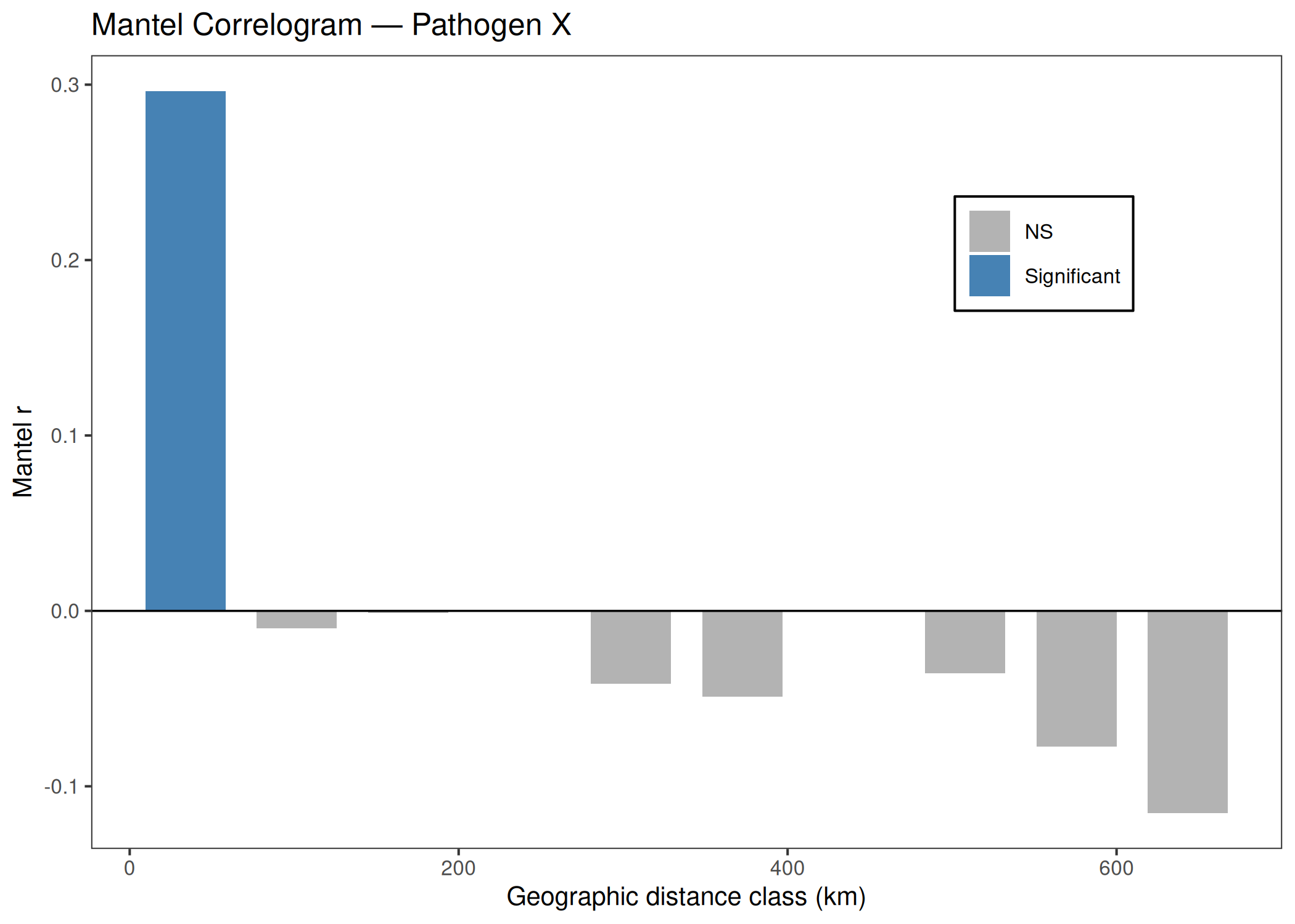
Mantel Correlogram

Code

# Distance class boundaries (km) — adjust to your study area
dist_breaks <- quantile(as.vector(geo_sub[lower.tri(geo_sub)]),
                         probs = seq(0, 1, by = 0.25))

# Mantel correlogram (vegan)
mcor <- mantel.correlog(
  D.eco  = pat_sub,
  D.geo  = geo_sub,
  nperm  = MANTEL_NPERM,
  cutoff = FALSE
)

mcor_df <- as.data.frame(mcor$mantel.res, check.names = FALSE)

# vegan reports raw and, when mult != "none", corrected p-values.
# Match the package's own plotting behavior by preferring corrected p-values.
p_col <- if ("Pr(corrected)" %in% names(mcor_df)) "Pr(corrected)" else "Pr(Mantel)"

mcor_df <- mcor_df %>%
  mutate(
    pvalue = .data[[p_col]],
    sig = ifelse(!is.na(pvalue) & pvalue <= 0.05, "Significant", "NS")
  )

p_mcor <- ggplot(mcor_df, aes(x = `class.index`, y = Mantel.cor, fill = sig)) +
  geom_bar(stat = "identity", width = diff(range(mcor_df$`class.index`)) / nrow(mcor_df) * 0.8) +
  geom_hline(yintercept = 0, color = "black", linewidth = 0.4) +
  scale_fill_manual(values = c("Significant" = "steelblue", "NS" = "grey70"),
                    name = NULL) +
  labs(title = paste("Mantel Correlogram —", PATHOGEN_NAME),
       x = "Geographic distance class (km)",
       y = "Mantel r") +
  theme_bw(base_size = 10, base_family = "sans") +
  theme(
    legend.position = c(0.8, 0.75),
    legend.background = element_rect(color = "black"),
    legend.key = element_rect(fill = "transparent"),
    panel.grid.major = element_blank(),
    panel.grid.minor = element_blank()
  )

ggsave(file.path(OUTPUT_DIR, "Mantel", "mantel_correlogram.tiff"),
       plot = p_mcor, width = 3, height = 2, dpi = 300,
       device = "tiff", compression = "lzw")
print(p_mcor)