04 · MagPix / Luminex Multiplex

2×2 factorial cytokine analysis with FDR correction and four plot types

immunology
luminex
ANOVA
multiplex

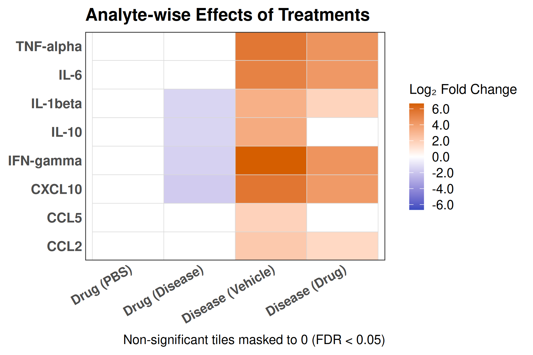
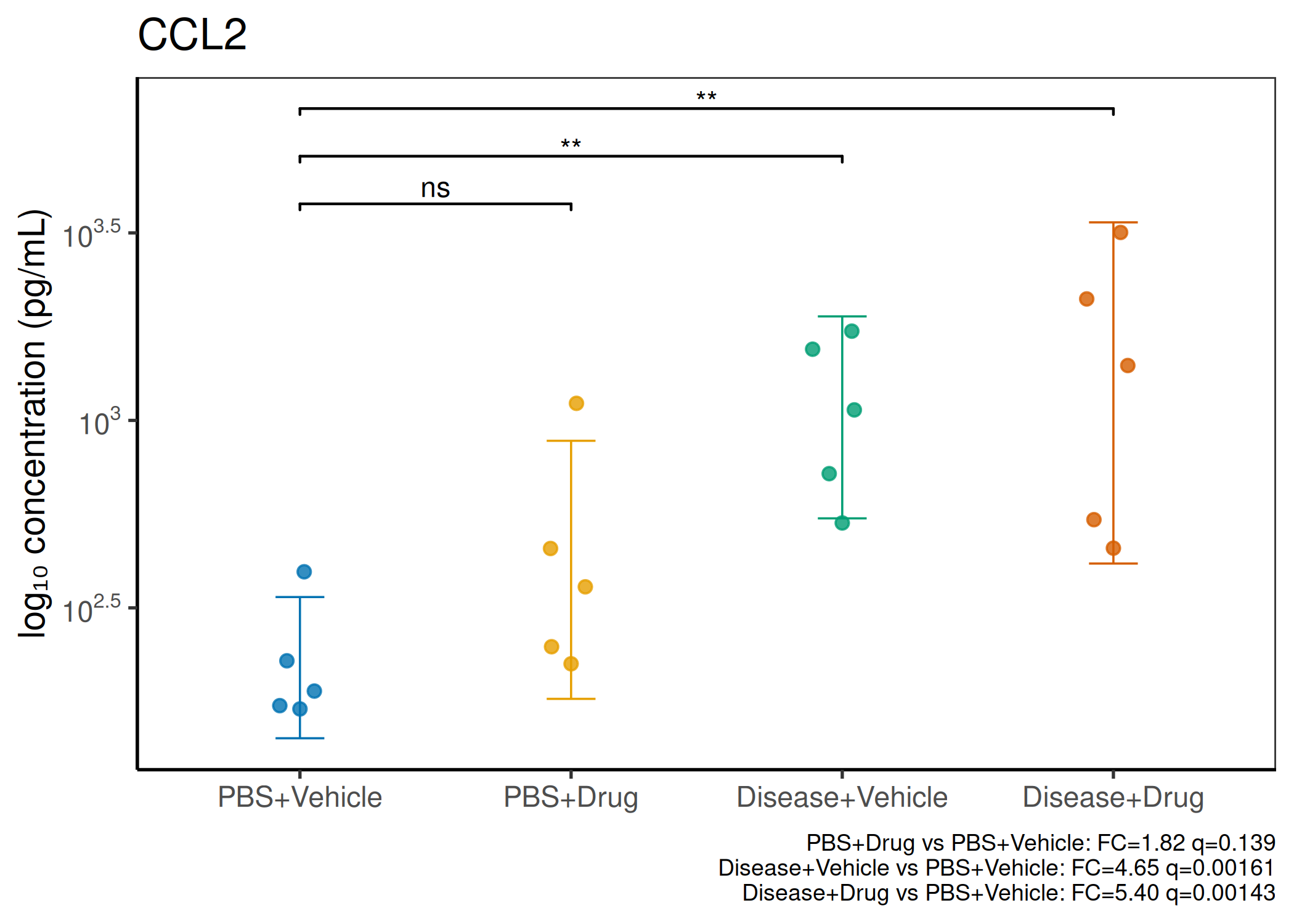
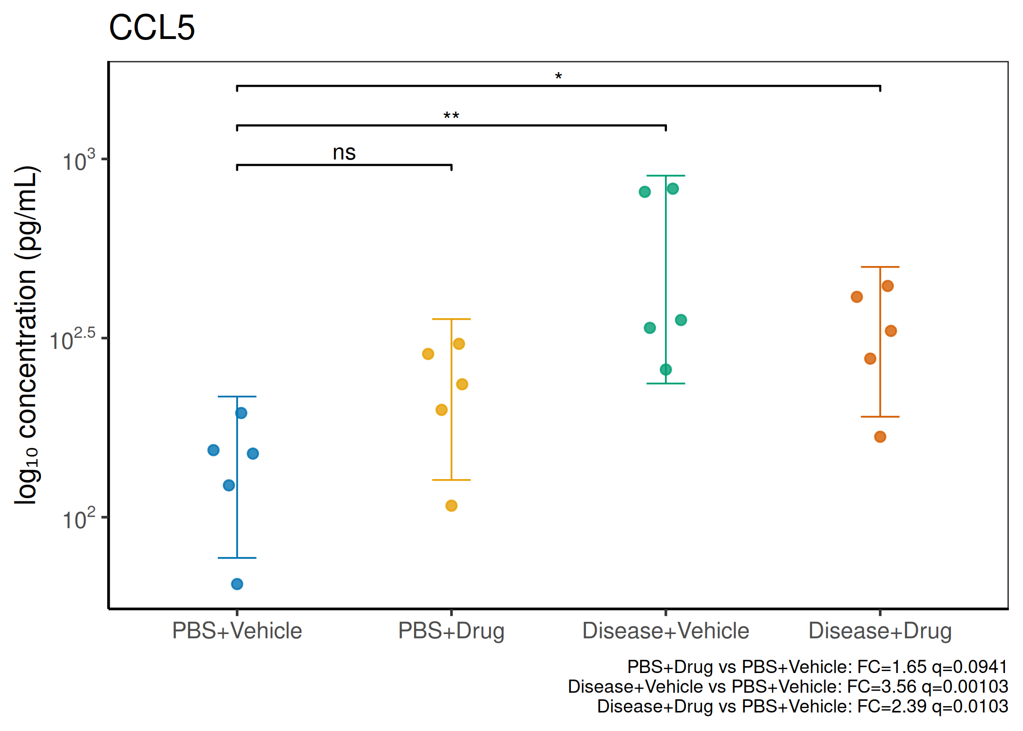
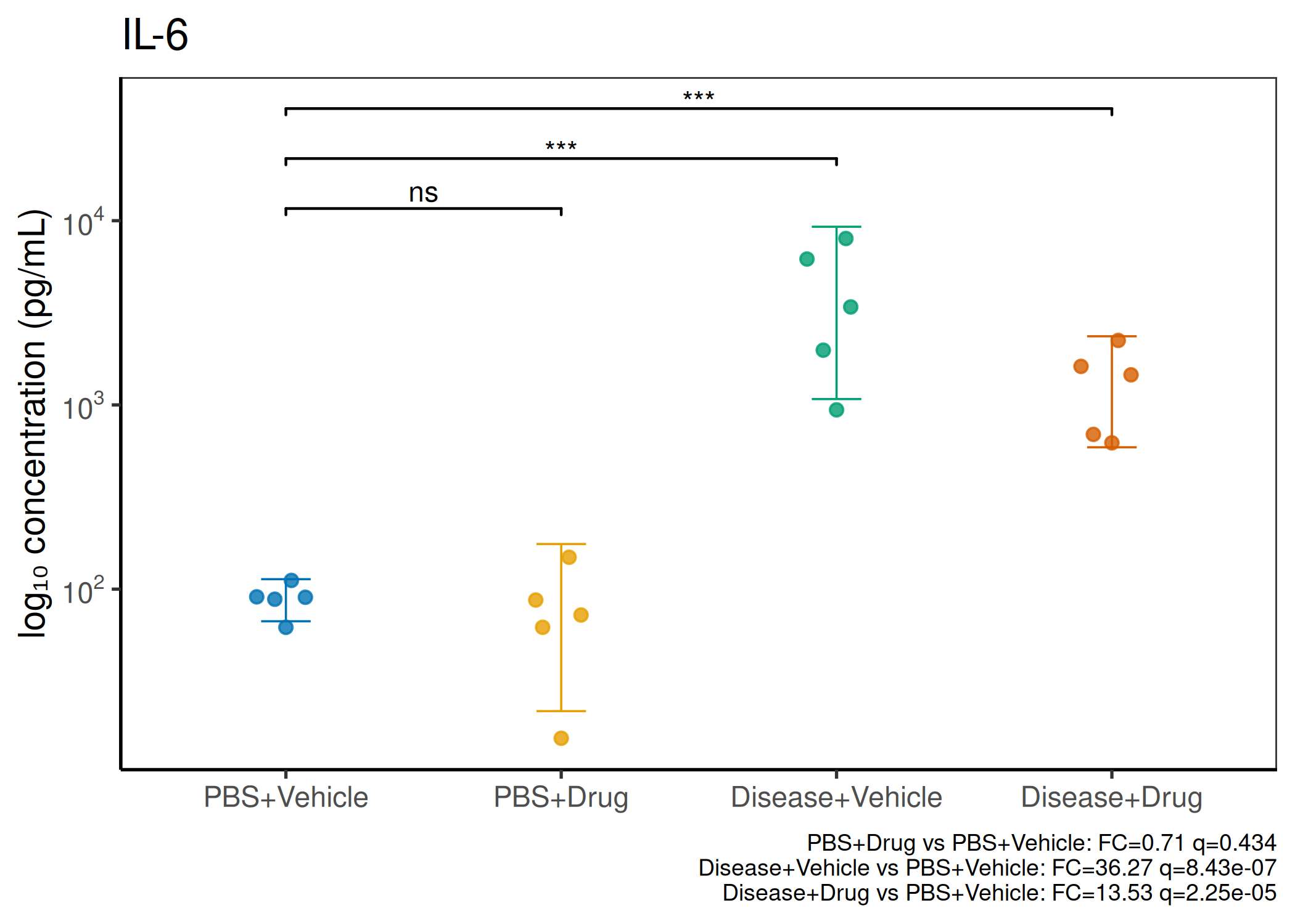
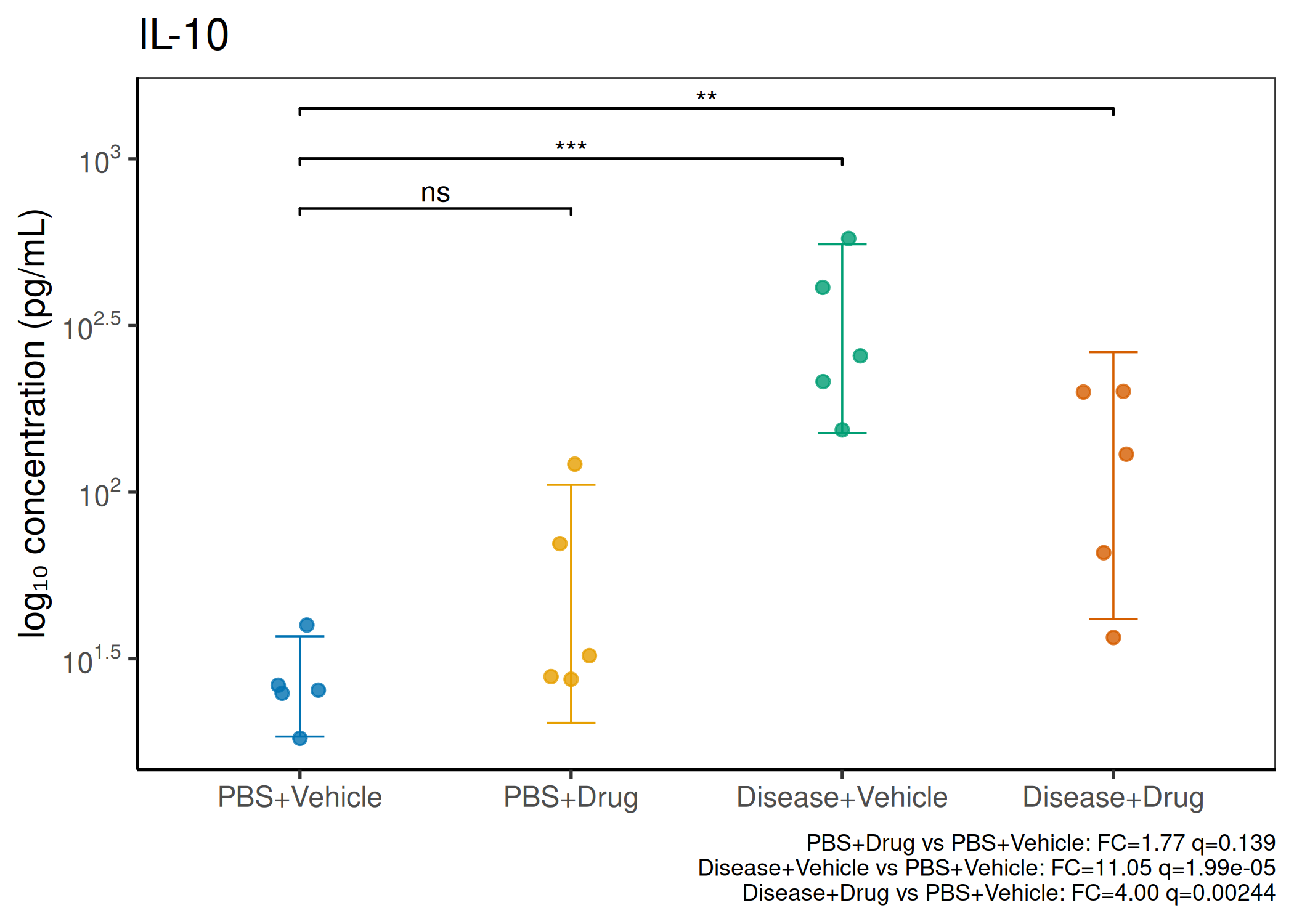
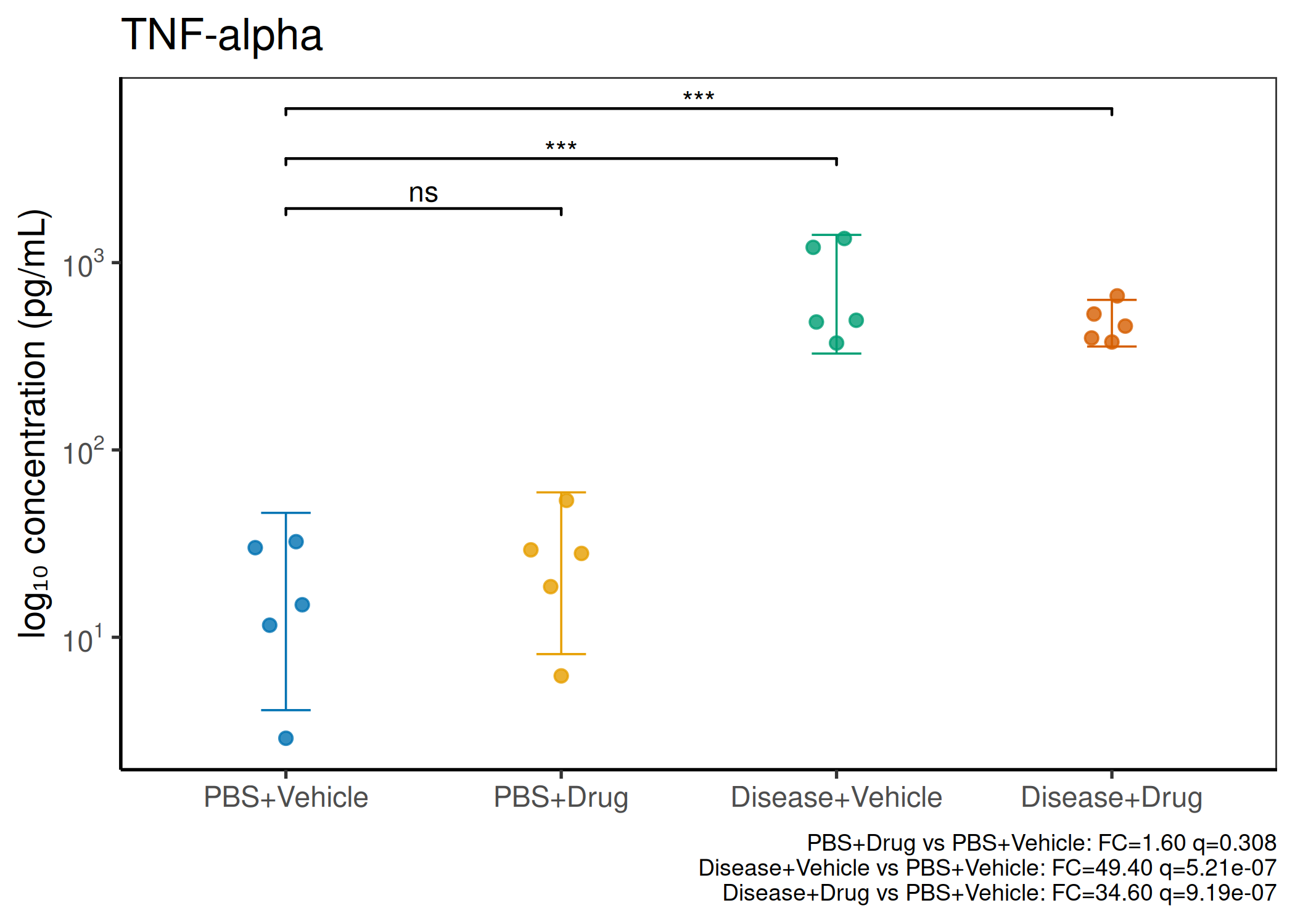
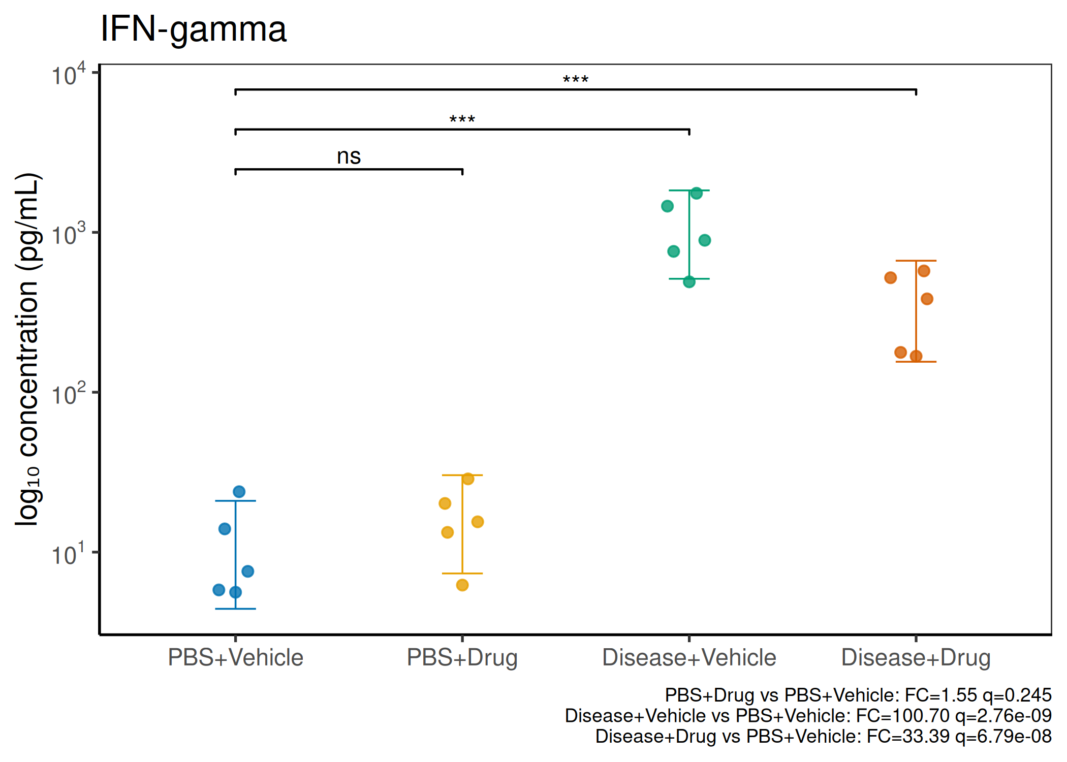
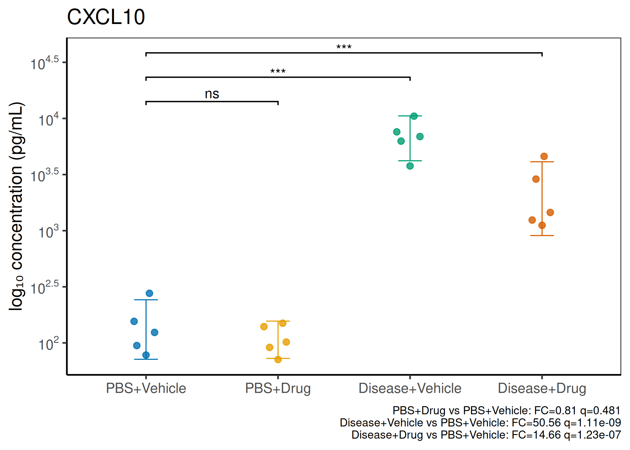
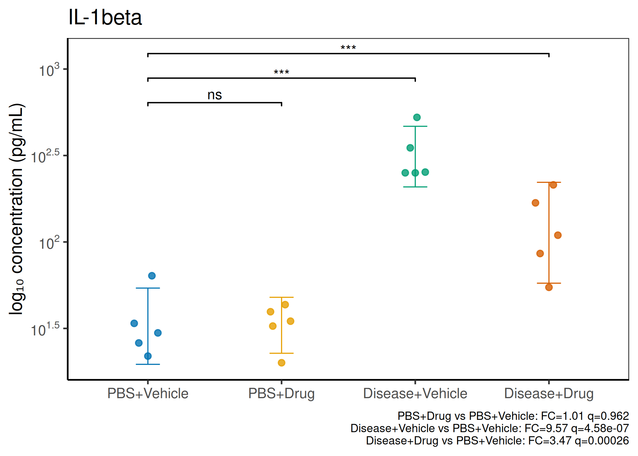
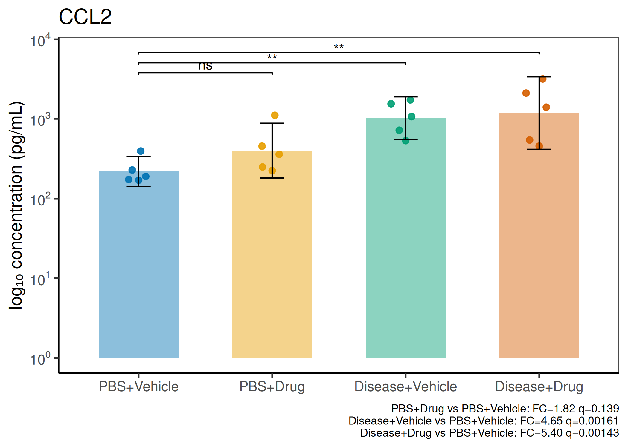
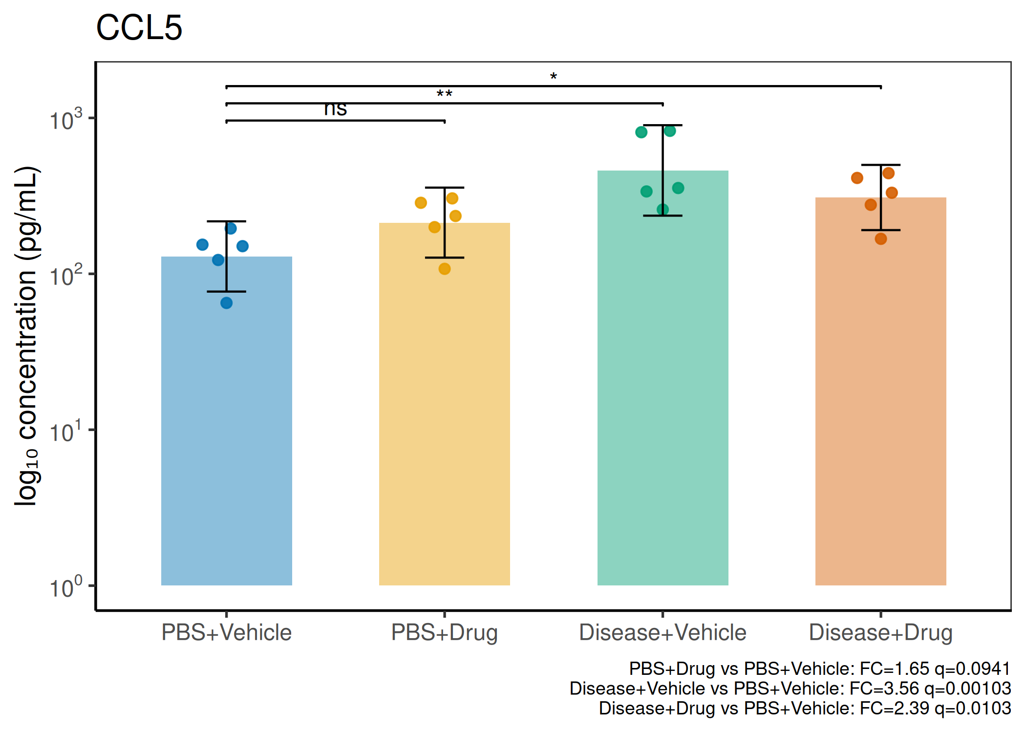
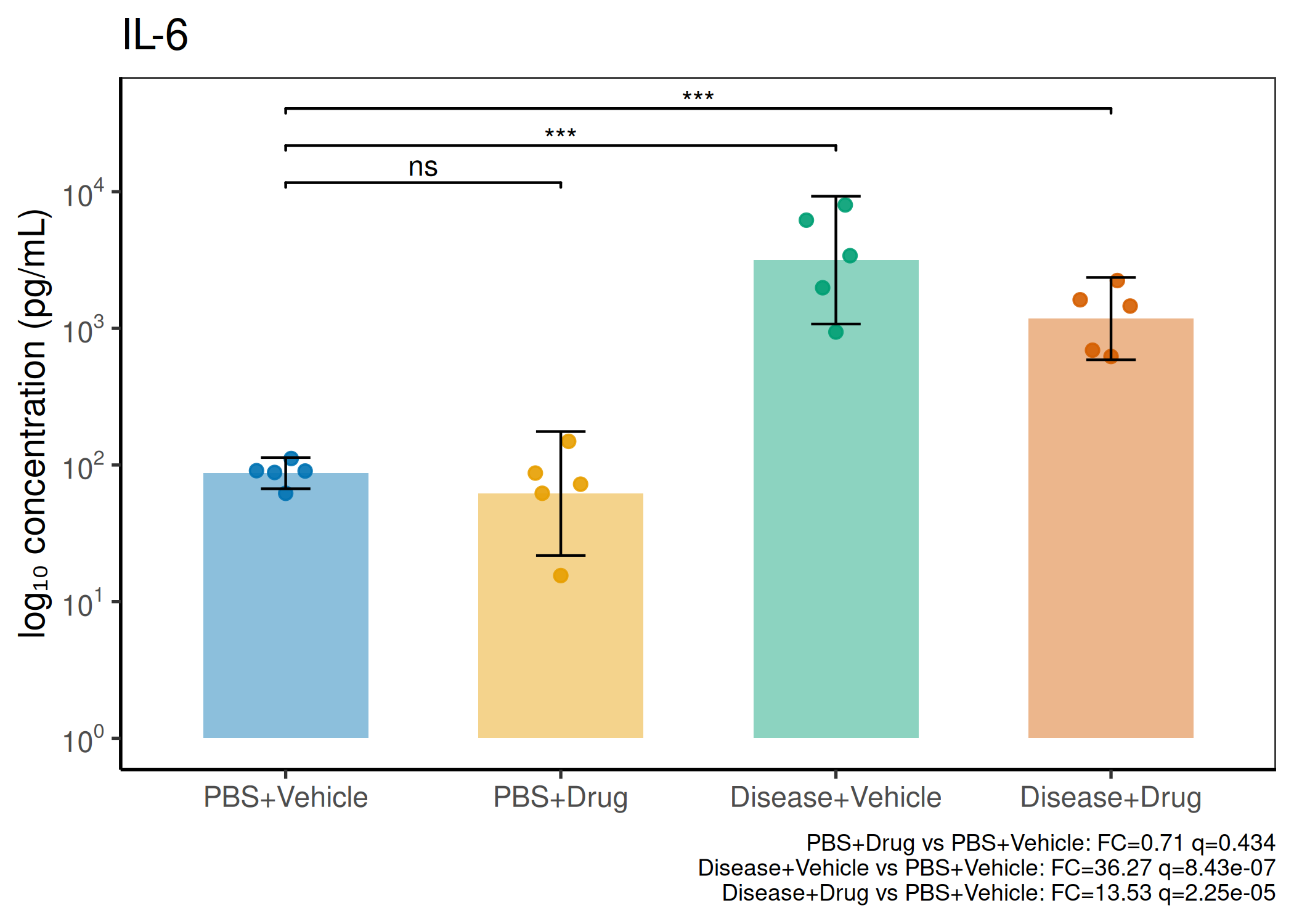
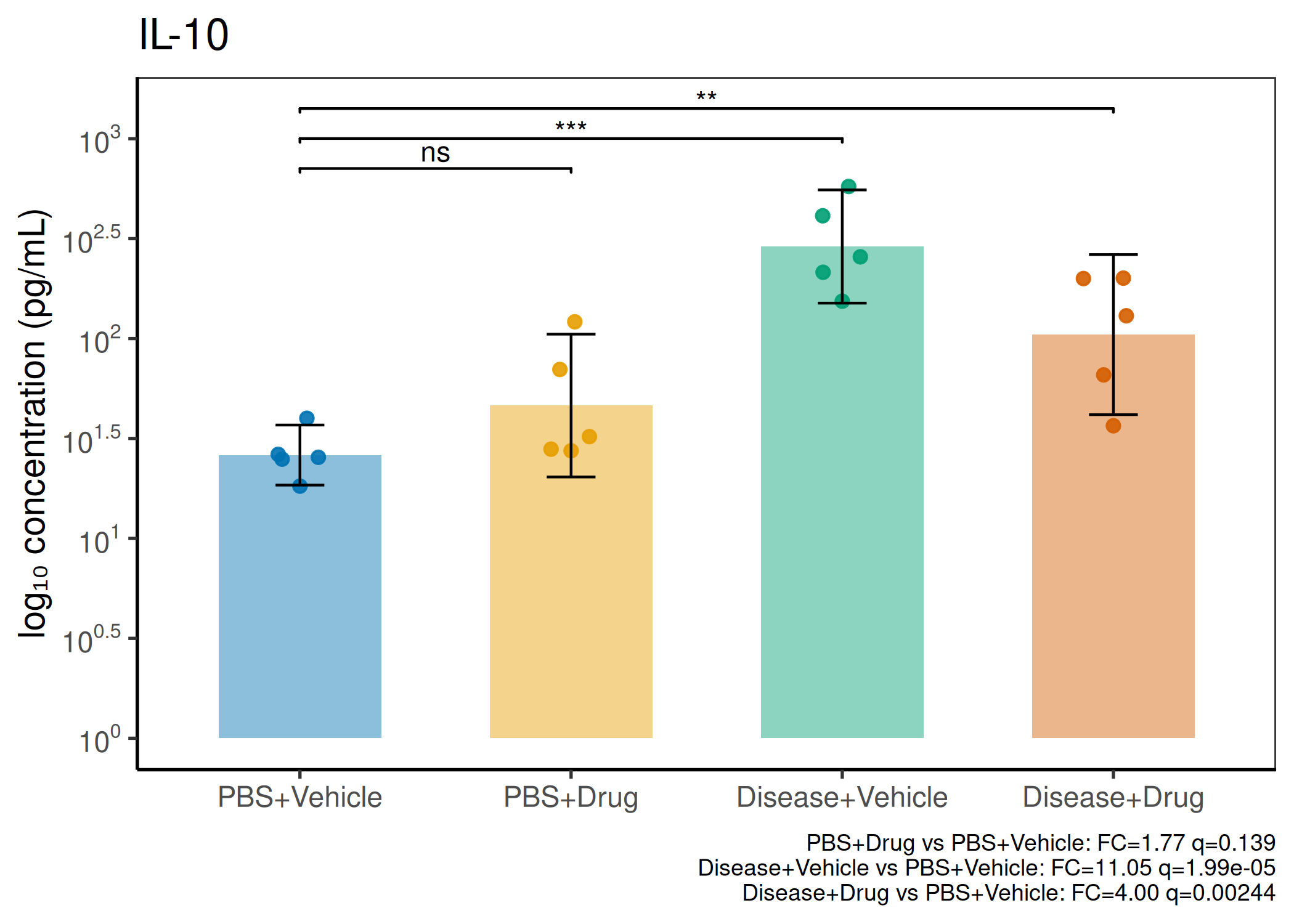
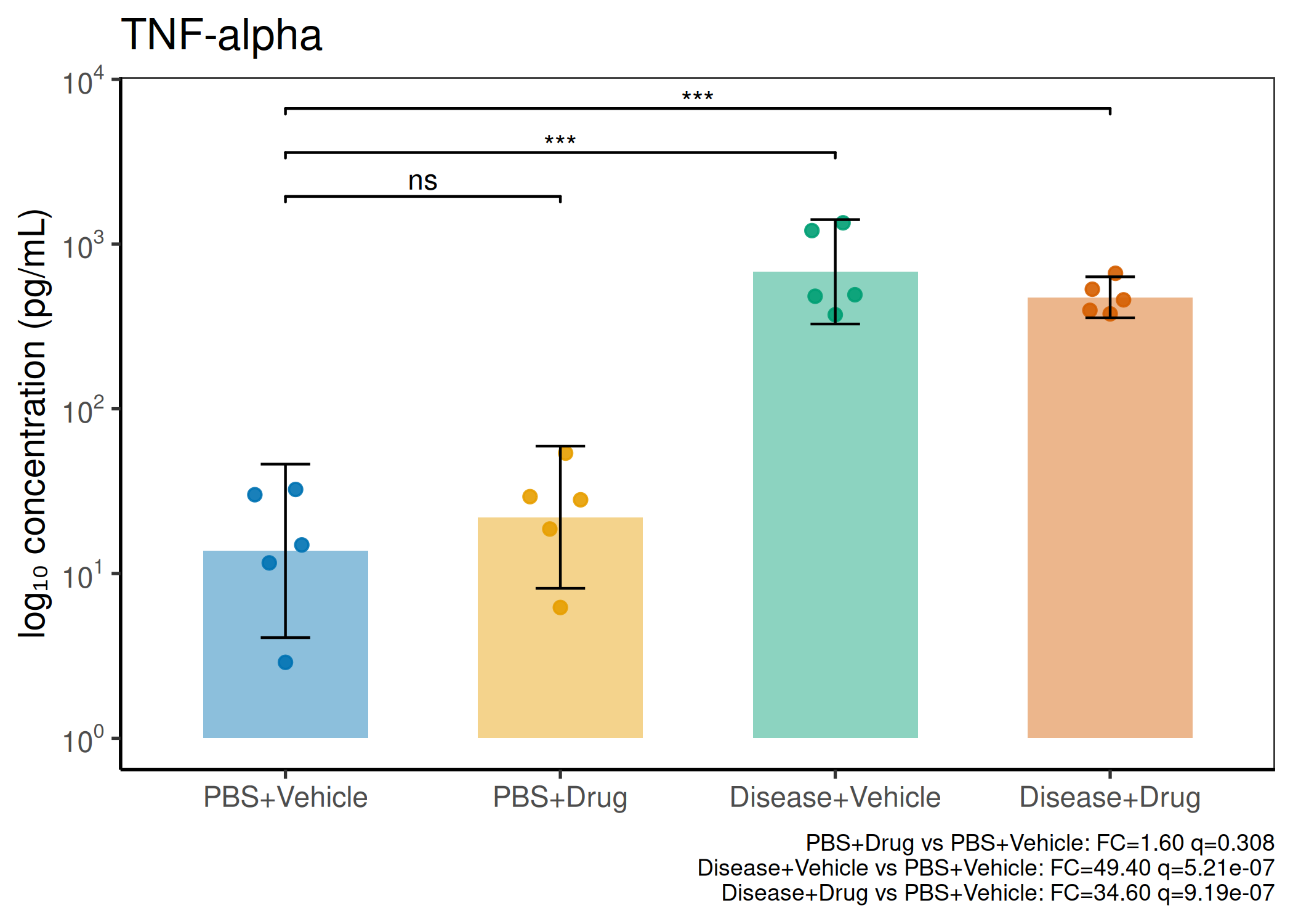
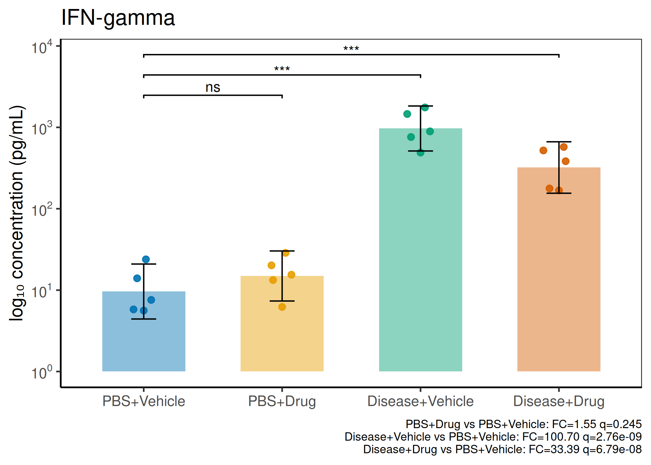
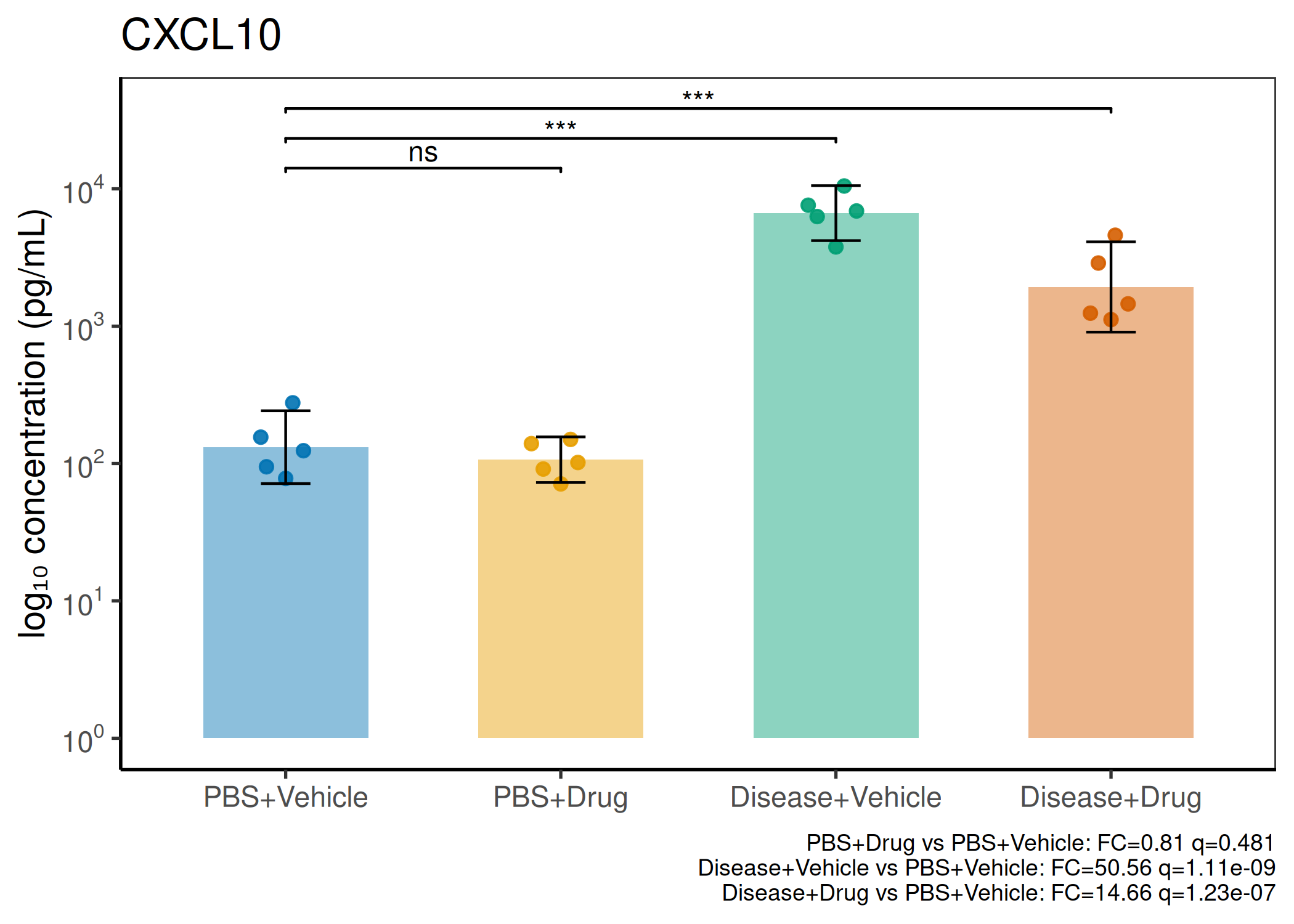
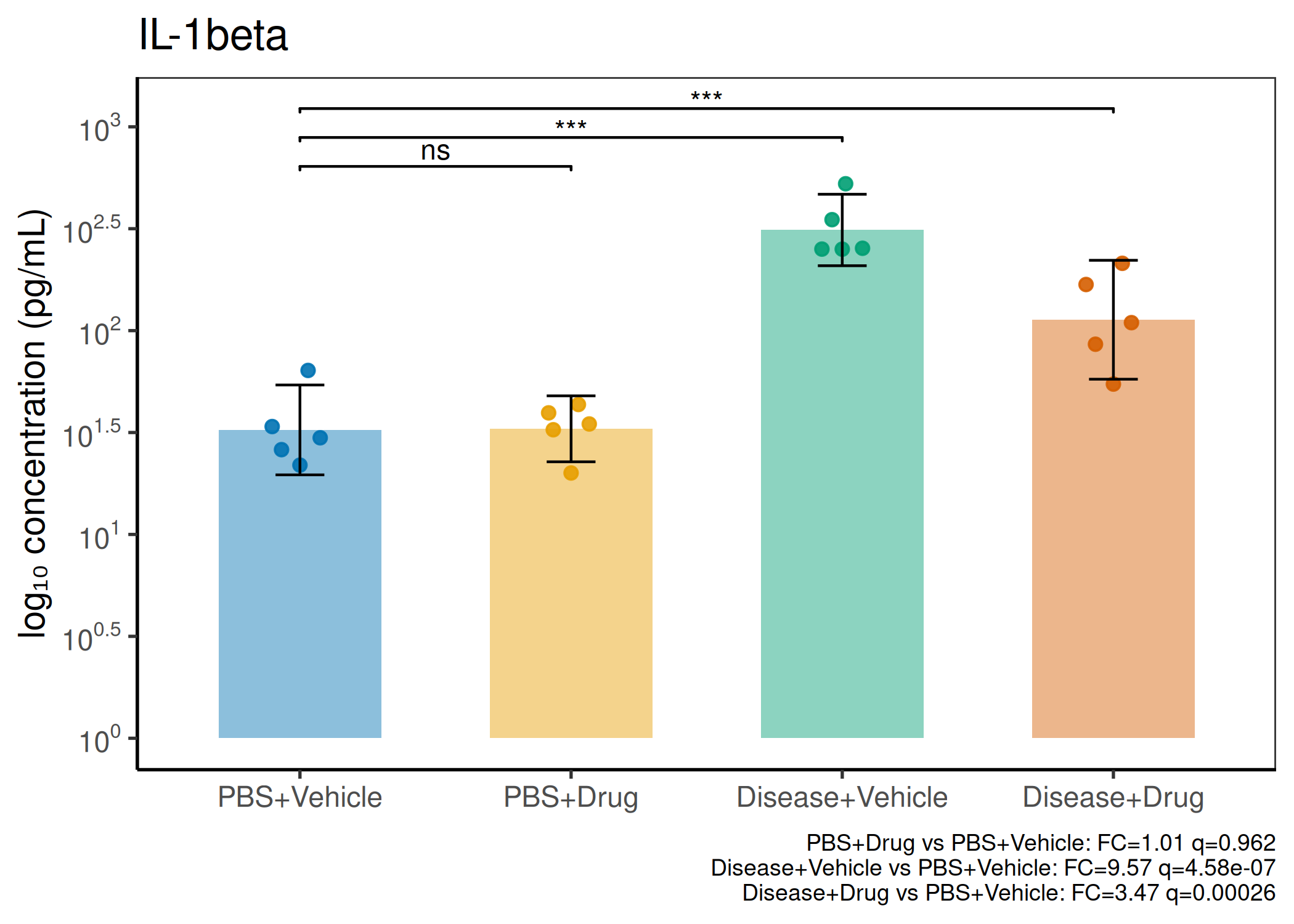
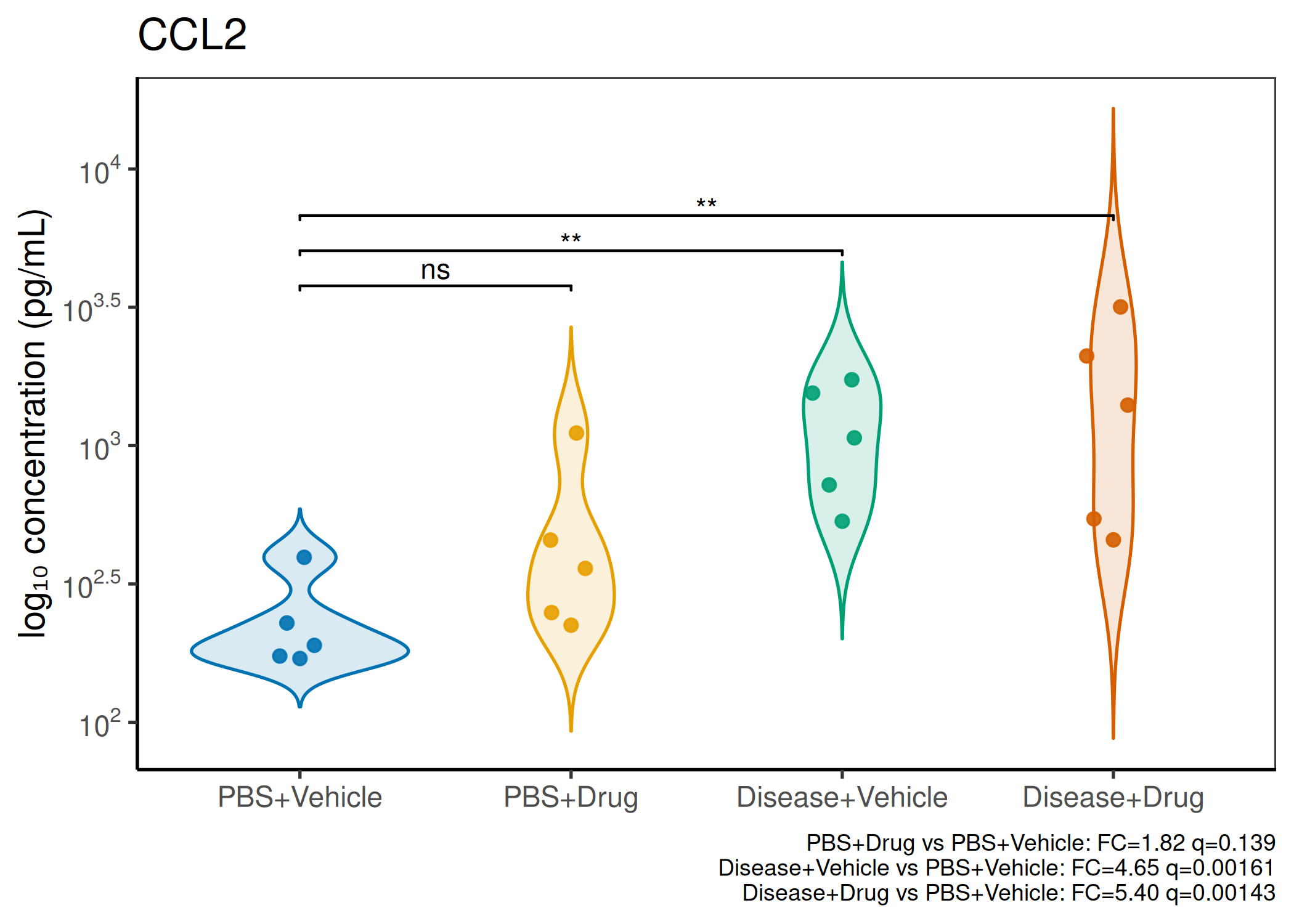
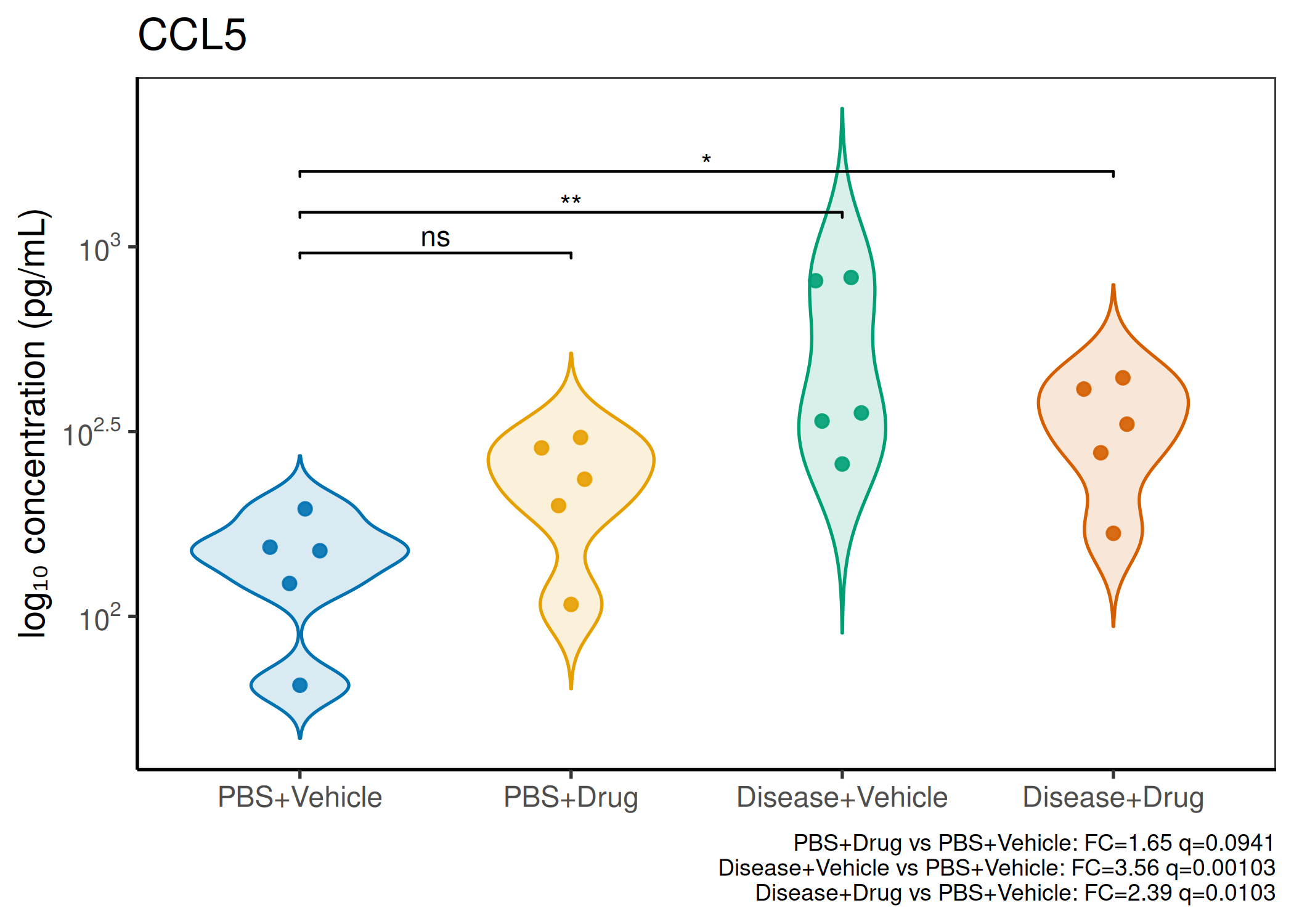
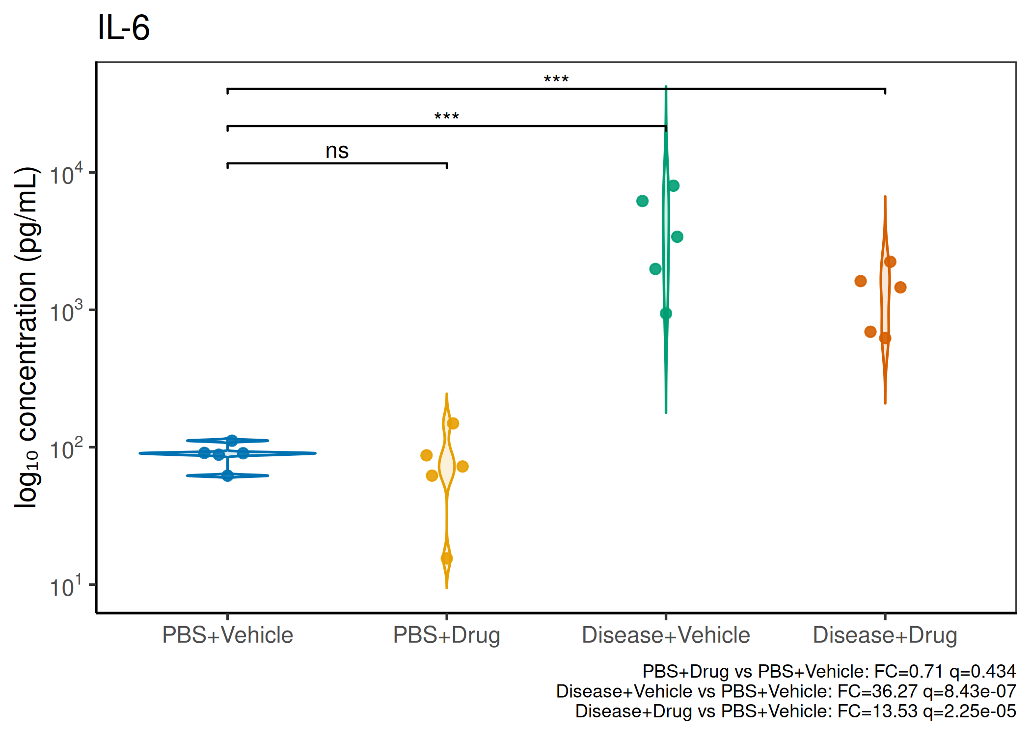
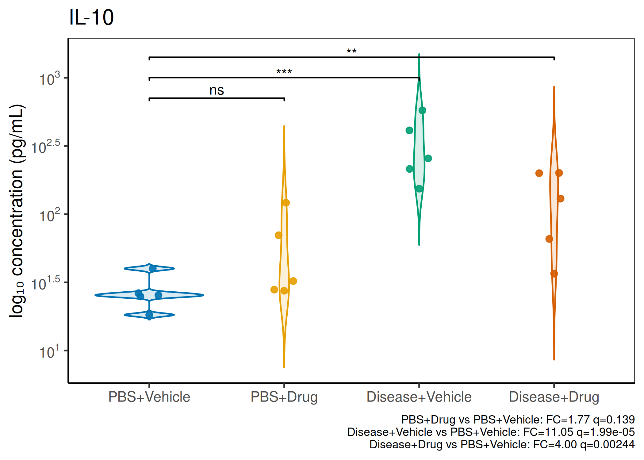
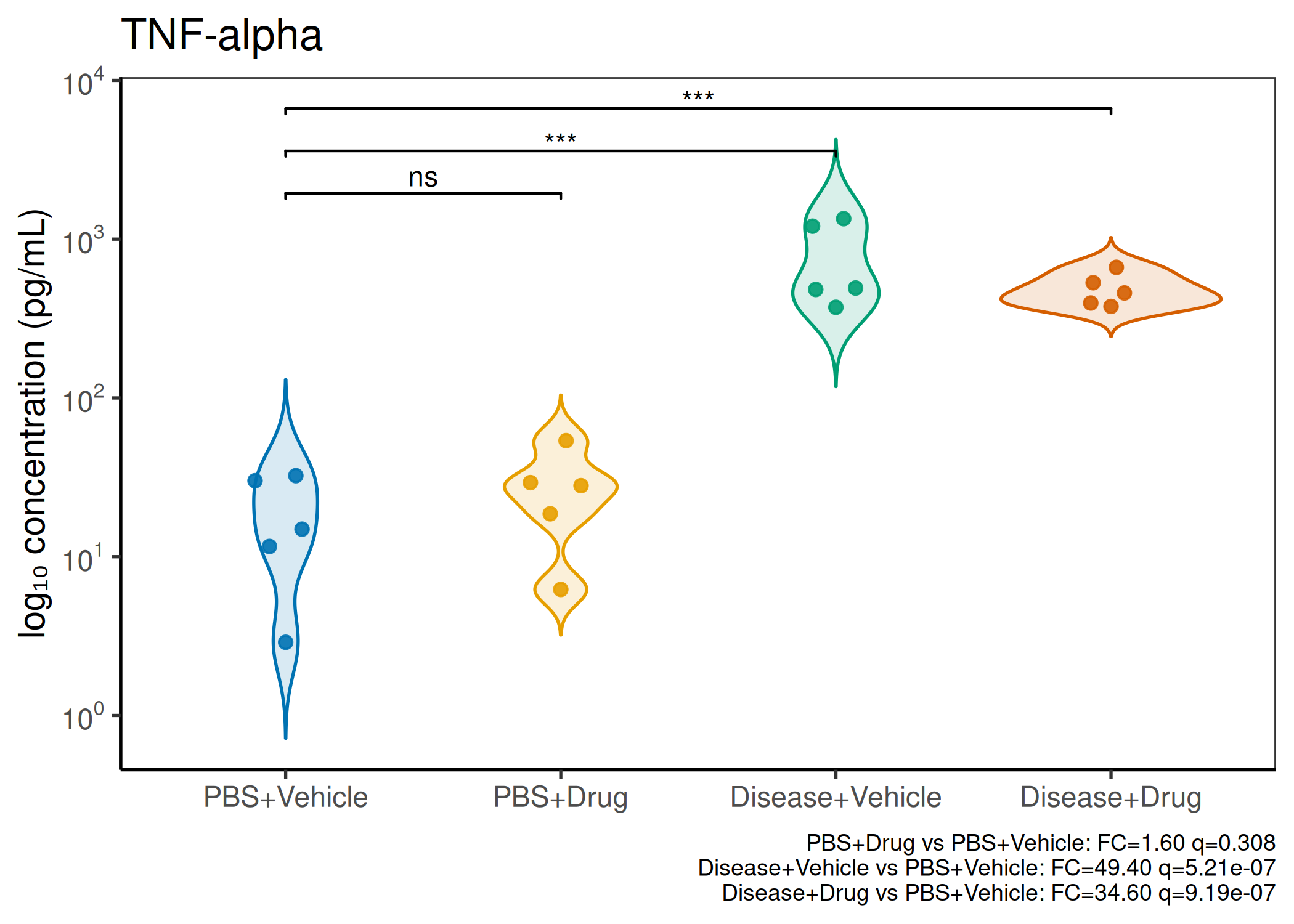
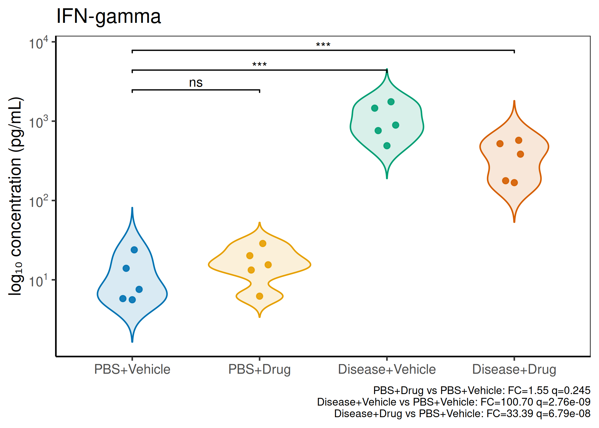
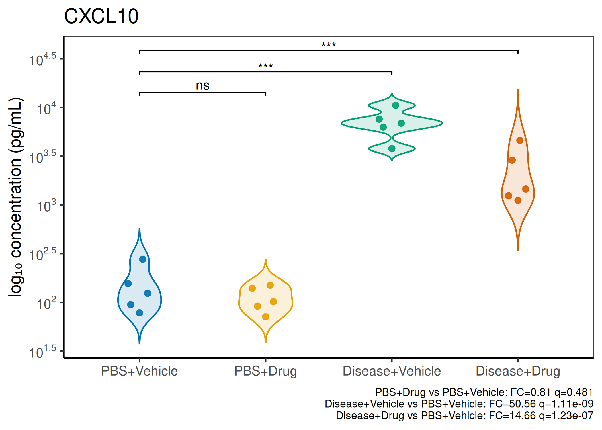
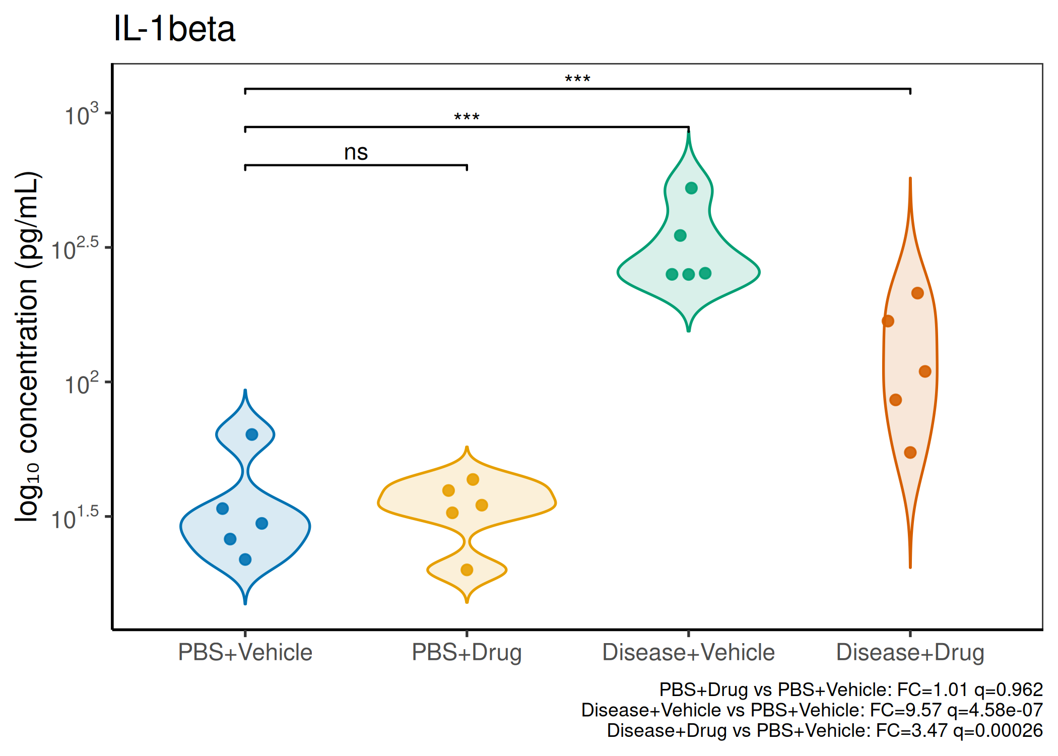
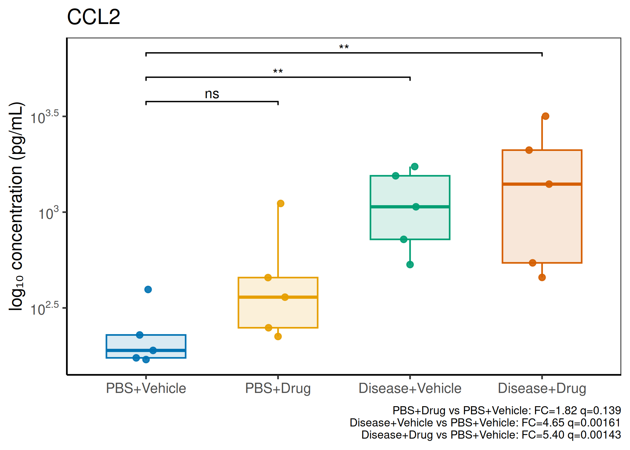
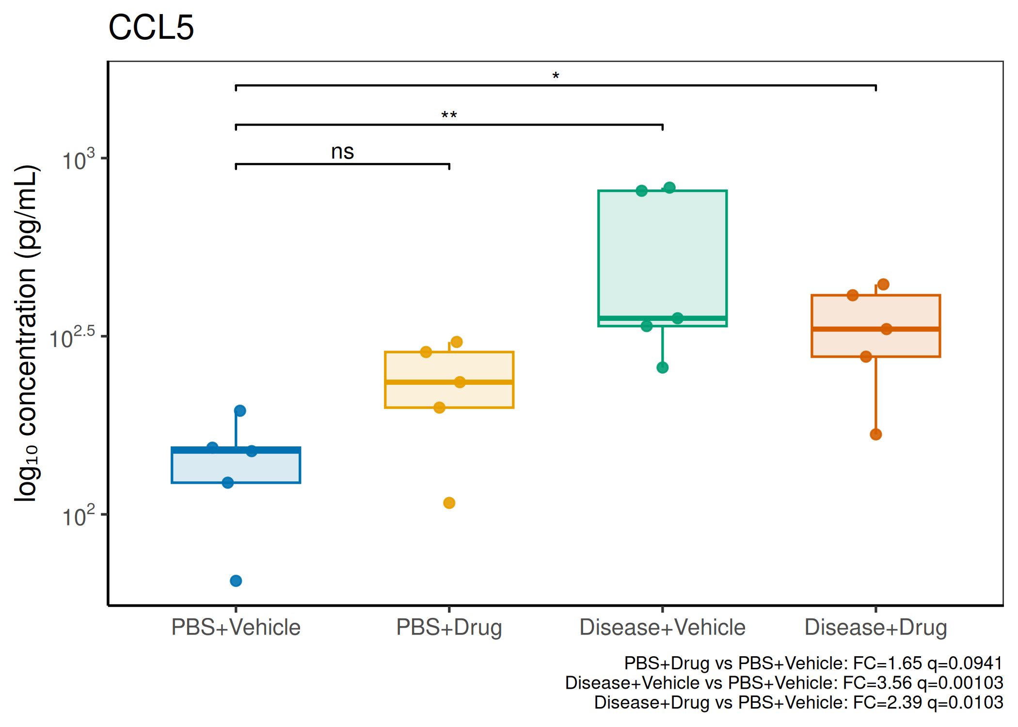
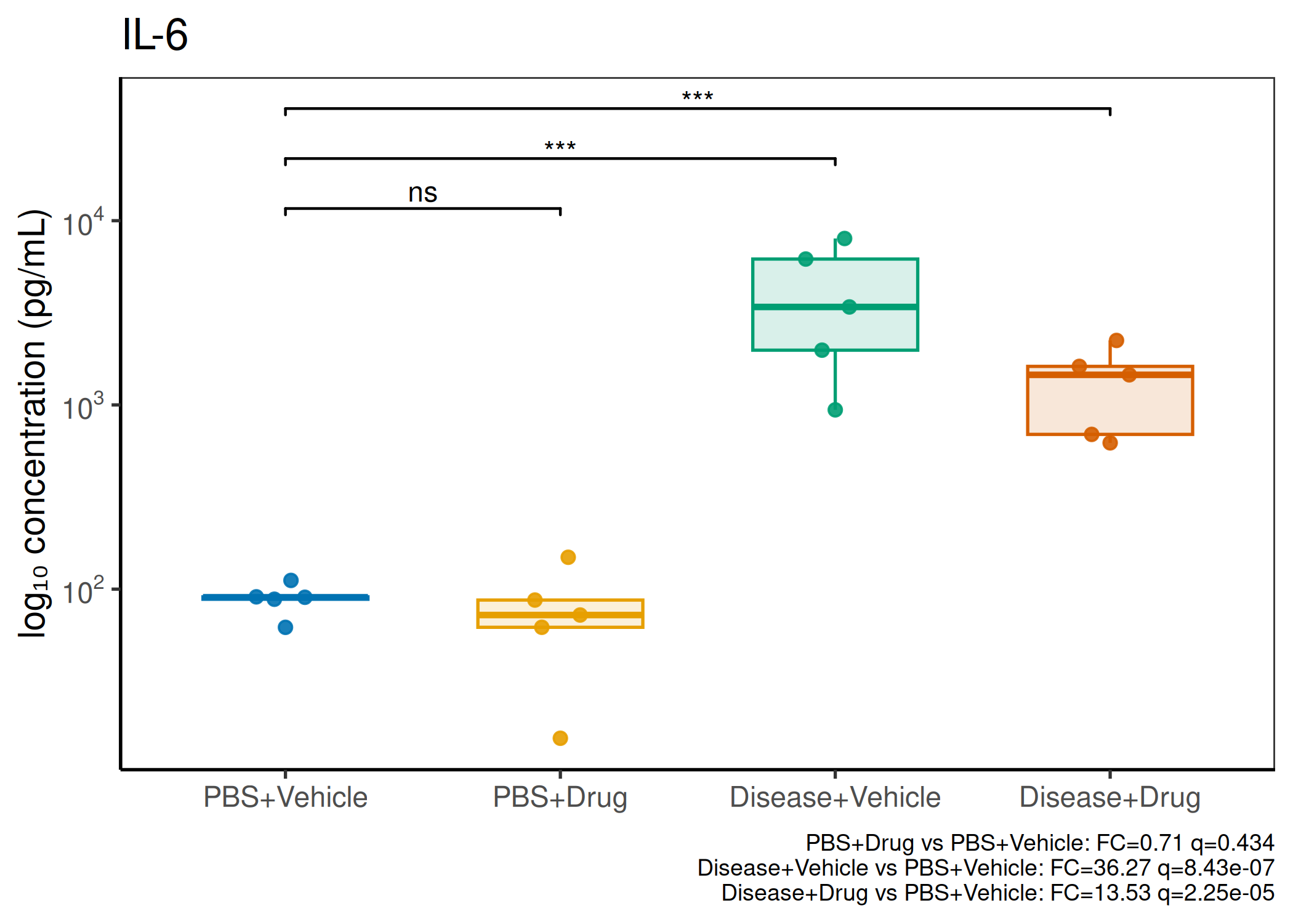
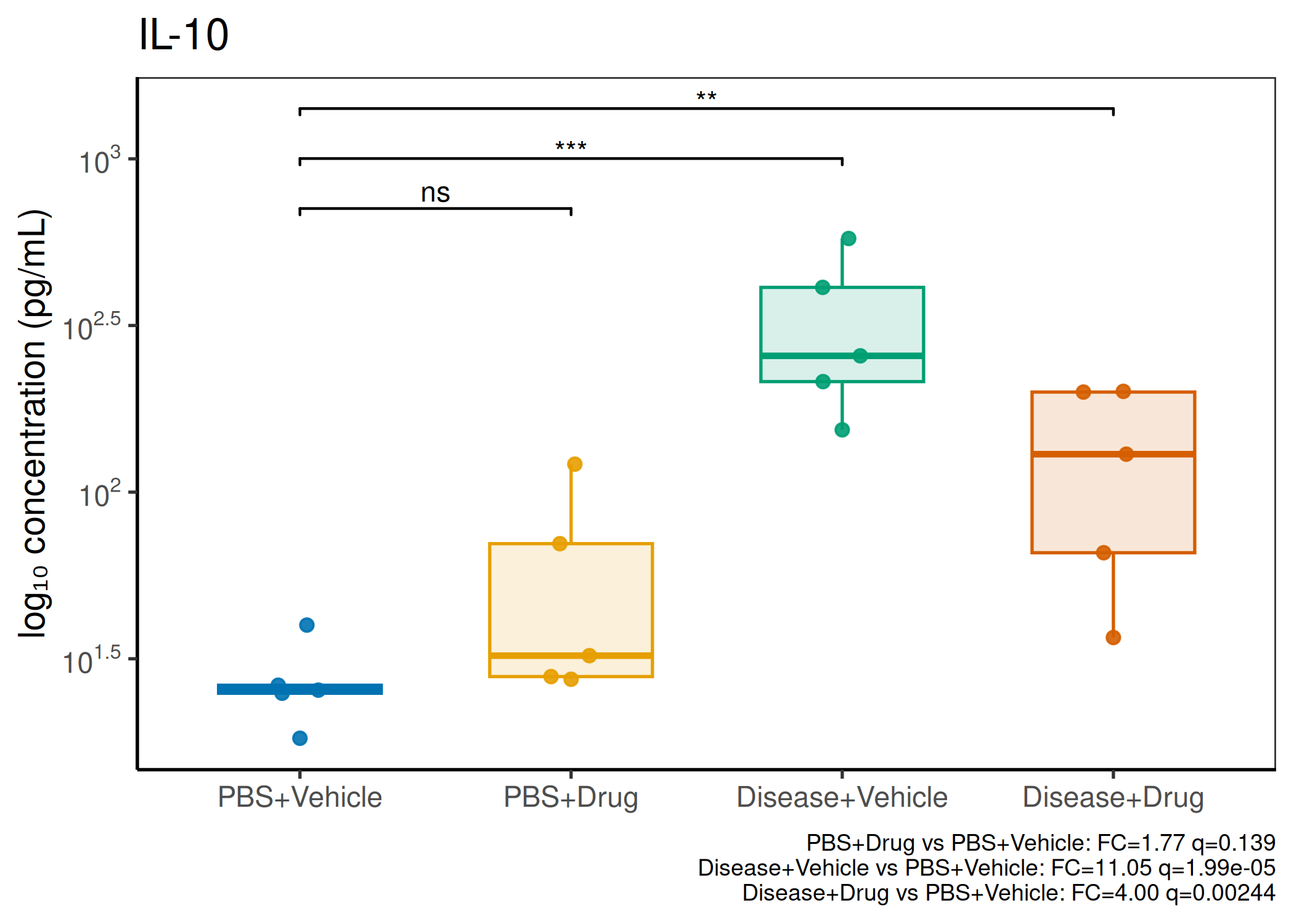
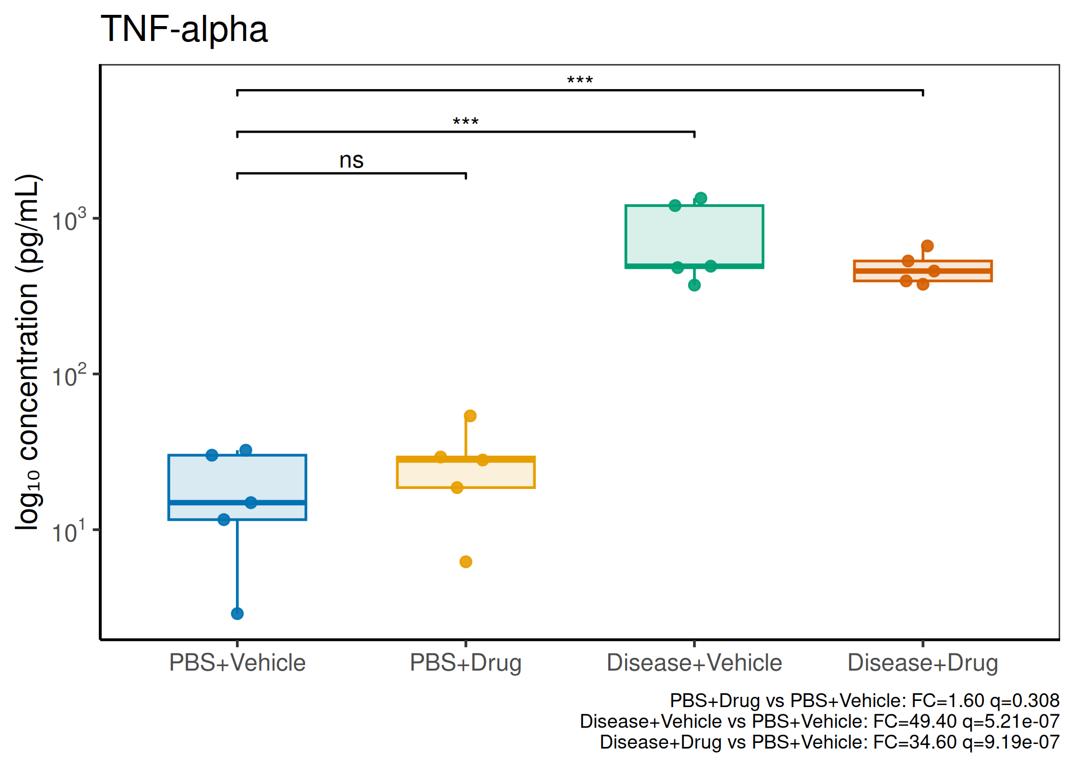
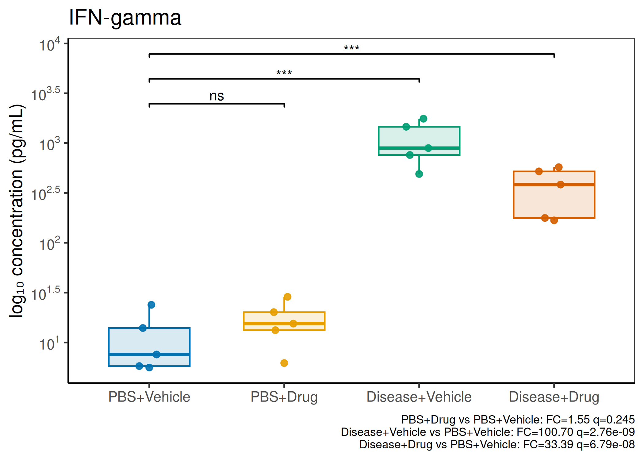
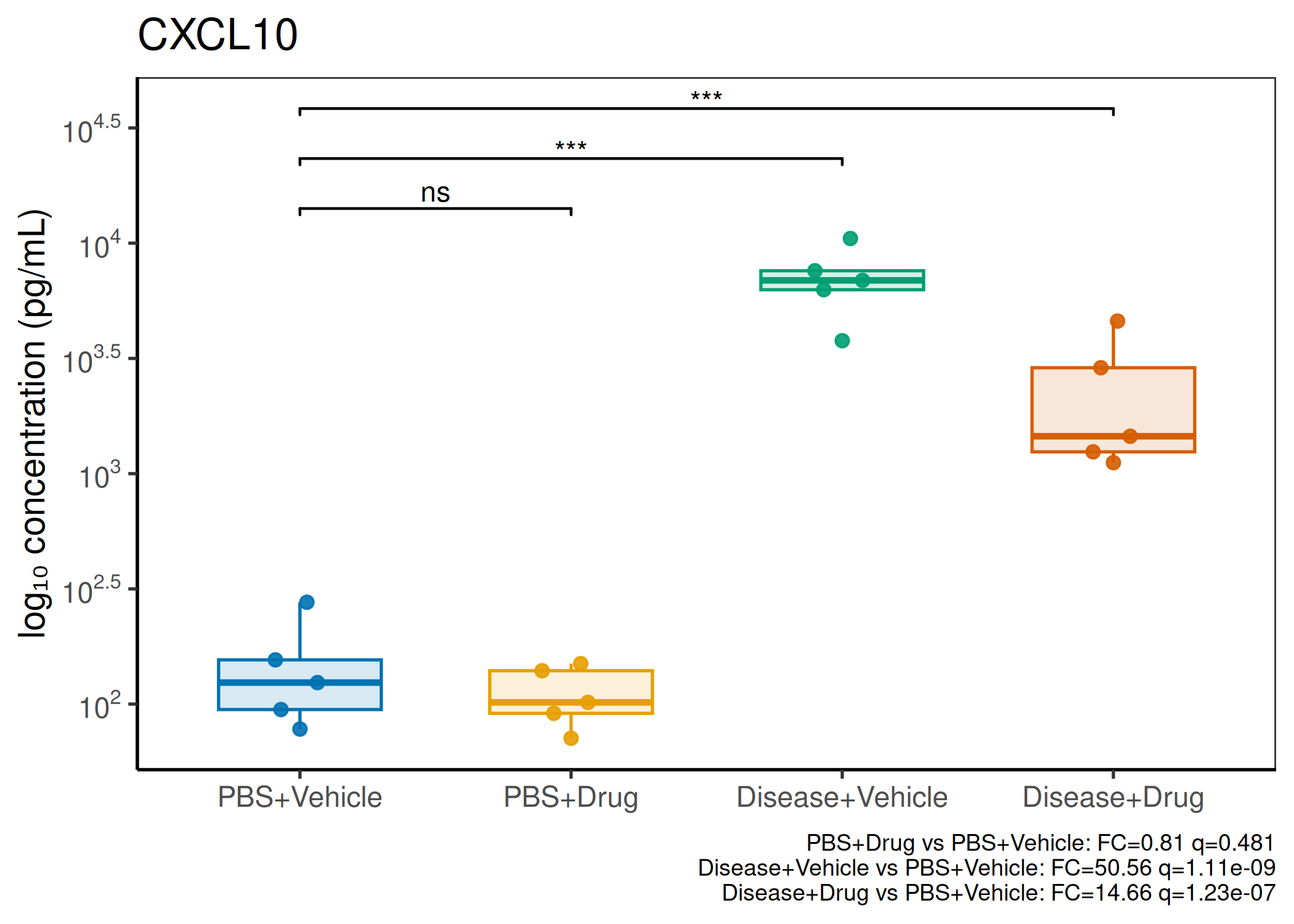
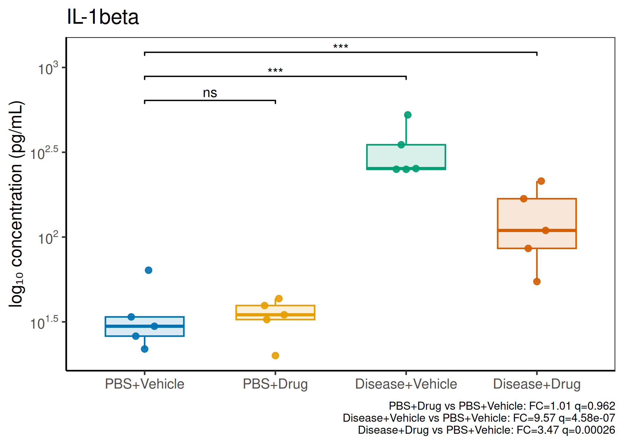
Analyzes multiplex immunoassay (MagPix/Luminex) data from a 2×2 factorial design (e.g., disease × treatment). Handles censored values (< LoD) via LoD/√2 substitution, flags outliers (3×IQR), fits per-analyte two-way ANOVA, computes emmeans contrasts with BH-FDR, and produces a heatmap plus four per-analyte plot types (dot, bar, violin, box).

Overview

Item Details
Input Single wide-format CSV (rows = samples, columns = analytes + metadata)
Key packages tidyverse, emmeans, ggbeeswarm, ggpubr, scales
Statistics Two-way ANOVA per analyte · emmeans contrasts · BH/FDR
Output QC tables · ANOVA results CSV · Contrasts CSV · Heatmap · 4 plot types per analyte
Download template.Rmd
Tip

When to use this template: You have a MagPix/Luminex panel run on a 2×2 factorial experiment (e.g., disease status × treatment). Adapt FACTOR1_LEVELS and FACTOR2_LEVELS to your own factor names.

Note

Okabe-Ito palette is used throughout — colorblind-safe for all four groups.

Back to Gallery Open Template File

Code
## ── USER CONFIGURATION ──────────────────────────────────────────────────────
#
# DATA_FILE: Path to your MagPix/Luminex export CSV.
#   Required columns (in addition to analyte columns):
#   - "Location"     : well identifier (e.g., "A1")
#   - "Sample"       : sample name — used to derive Factor1 and Factor2
#   - "Original_ID"  : original sample ID (can be same as Sample)
#   - "Total Events" : bead event count (for QC)
#
DATA_FILE <- "data/luminex_data.csv"

# NON_ANALYTE_COLS: Columns that are NOT cytokine measurements.
#   All other columns will be treated as analytes.
NON_ANALYTE_COLS <- c("Location", "Sample", "Original_ID", "Total Events")

# FACTOR1_PATTERN / FACTOR2_PATTERN: Regex patterns matched against the
#   Sample column to assign Factor1 and Factor2.
#   The default detects "<name>" at start-of-string for Factor1,
#   and "<name>" anywhere for Factor2.
#
#   Example: Sample = "Disease_Drug_1"
#     FACTOR1_LEVELS[2] = "Disease" → if str_detect(Sample, "Disease") → "Disease"
#     FACTOR2_LEVELS[2] = "Drug"    → if str_detect(Sample, "Drug")    → "Drug"
#
FACTOR1_LEVELS <- c("PBS", "Disease")     # [1] = reference / control level
FACTOR2_LEVELS <- c("Vehicle", "Drug")    # [1] = reference / control level

# BASELINE_GROUP: The reference group label for emmeans contrasts.
#   Format: "<FACTOR1_ref>+<FACTOR2_ref>"
BASELINE_GROUP <- paste0(FACTOR1_LEVELS[1], "+", FACTOR2_LEVELS[1])

# OKABE_ITO: Colorblind-safe 4-color palette for the four 2×2 groups.
#   Names follow the "<Factor1>+<Factor2>" convention.
OKABE_ITO <- c(
  "PBS+Vehicle"      = "#0072B2",   # Blue
  "PBS+Drug"         = "#E69F00",   # Orange
  "Disease+Vehicle"  = "#009E73",   # Bluish green
  "Disease+Drug"     = "#D55E00"    # Vermilion
)

# CONTRAST_ORDER / CONTRAST_LABELS: Define which emmeans contrasts appear in
#   the heatmap (order matters for the y-axis) and their display labels.
#   Adjust if your Factor levels produce different contrast names.
CONTRAST_ORDER <- c(
  paste0(FACTOR2_LEVELS[2], " - ", FACTOR2_LEVELS[1], ", ", FACTOR1_LEVELS[1]),
  paste0(FACTOR2_LEVELS[2], " - ", FACTOR2_LEVELS[1], ", ", FACTOR1_LEVELS[2]),
  paste0(FACTOR1_LEVELS[2], " - ", FACTOR1_LEVELS[1], ", ", FACTOR2_LEVELS[1]),
  paste0(FACTOR1_LEVELS[2], " - ", FACTOR1_LEVELS[1], ", ", FACTOR2_LEVELS[2])
)
CONTRAST_LABELS <- c(
  paste0("Drug (", FACTOR1_LEVELS[1], ")"),
  paste0("Drug (", FACTOR1_LEVELS[2], ")"),
  paste0(FACTOR1_LEVELS[2], " (", FACTOR2_LEVELS[1], ")"),
  paste0(FACTOR1_LEVELS[2], " (", FACTOR2_LEVELS[2], ")")
)

# OUTPUT_DIR: Folder where per-analyte plots are saved.
OUTPUT_DIR <- "Plots"

## ────────────────────────────────────────────────────────────────────────────

MagPix / Luminex Best Practices

  • Bead counts: ≥35 per analyte (≥50 ideal). Re-export with bead counts if missing.
  • Censoring (“< LoD”): Do not treat as zero. Replace with LoD/√2 for substitution.
  • QC/outliers: Flag wells using Tukey 3×IQR on the log10 scale.
  • Design: 2×2 factorial — model on log10(concentration), test main effects and interaction.
  • Multiple analytes: Correct FDR across analytes (BH). Report fold-changes as 10^β.

Setup

Code
library(tidyverse)
library(stringr)
library(broom)
library(emmeans)
library(ggpubr)
library(ggbeeswarm)
library(scales)
library(forcats)

Load Data

Code
raw <- read_csv(DATA_FILE, show_col_types = FALSE)

analyte_cols <- setdiff(names(raw), NON_ANALYTE_COLS)
raw <- raw %>% mutate(across(all_of(analyte_cols), as.character))

dat_long <- raw %>%
  pivot_longer(all_of(analyte_cols), names_to = "Analyte", values_to = "raw_value") %>%
  mutate(
    censored    = str_detect(raw_value, "^\\s*<"),
    above_ul    = str_detect(raw_value, "^\\s*>"),
    lod         = if_else(censored, parse_number(raw_value), NA_real_),
    value       = if_else(censored, lod / sqrt(2), parse_number(raw_value)),
    log10_value = log10(value),
    Factor1     = if_else(str_detect(Sample, FACTOR1_LEVELS[2]),
                          FACTOR1_LEVELS[2], FACTOR1_LEVELS[1]),
    Factor2     = if_else(str_detect(Sample, FACTOR2_LEVELS[2]),
                          FACTOR2_LEVELS[2], FACTOR2_LEVELS[1]),
    Factor1     = factor(Factor1, levels = FACTOR1_LEVELS),
    Factor2     = factor(Factor2, levels = FACTOR2_LEVELS),
    Group       = factor(
      paste0(Factor1, "+", Factor2),
      levels = paste0(
        rep(FACTOR1_LEVELS, each = 2),
        "+",
        rep(FACTOR2_LEVELS, times = 2)
      )
    )
  )

dat_long
# A tibble: 160 × 14
   Location Sample         Original_ID `Total Events` Analyte raw_value censored
   <chr>    <chr>          <chr>                <dbl> <chr>   <chr>     <lgl>   
 1 Row1     PBS_Vehicle_1  ID_1                   116 CCL2    228.47    FALSE   
 2 Row1     PBS_Vehicle_1  ID_1                   116 CCL5    195.34    FALSE   
 3 Row1     PBS_Vehicle_1  ID_1                   116 IL-6    90.83     FALSE   
 4 Row1     PBS_Vehicle_1  ID_1                   116 IL-10   39.91     FALSE   
 5 Row1     PBS_Vehicle_1  ID_1                   116 TNF-al… 14.91     FALSE   
 6 Row1     PBS_Vehicle_1  ID_1                   116 IFN-ga… 23.87     FALSE   
 7 Row1     PBS_Vehicle_1  ID_1                   116 CXCL10  94.7      FALSE   
 8 Row1     PBS_Vehicle_1  ID_1                   116 IL-1be… 63.77     FALSE   
 9 Row1     Disease_Vehic… ID_2                   105 CCL2    1729.63   FALSE   
10 Row1     Disease_Vehic… ID_2                   105 CCL5    337.65    FALSE   
# ℹ 150 more rows
# ℹ 7 more variables: above_ul <lgl>, lod <dbl>, value <dbl>,
#   log10_value <dbl>, Factor1 <fct>, Factor2 <fct>, Group <fct>

QC

Censoring Rate per Analyte

Code
qc_censor <- dat_long %>%
  group_by(Analyte) %>%
  summarise(
    n        = n(),
    cens_n   = sum(censored),
    cens_pct = 100 * cens_n / n,
    .groups  = "drop"
  ) %>%
  arrange(desc(cens_pct))

print(qc_censor, n = Inf)
# A tibble: 8 × 4
  Analyte       n cens_n cens_pct
  <chr>     <int>  <int>    <dbl>
1 CCL2         20      0        0
2 CCL5         20      0        0
3 CXCL10       20      0        0
4 IFN-gamma    20      0        0
5 IL-10        20      0        0
6 IL-1beta     20      0        0
7 IL-6         20      0        0
8 TNF-alpha    20      0        0

Guidance: Analytes with >50% censoring warrant Tobit regression as a sensitivity check. The standard substitution (LoD/√2) used here is appropriate for <30% censoring.

Outliers (Tukey 3×IQR on log10 scale)

Code
fences <- dat_long %>%
  group_by(Analyte) %>%
  summarise(
    q1    = quantile(log10_value, 0.25, na.rm = TRUE),
    q3    = quantile(log10_value, 0.75, na.rm = TRUE),
    iqr   = IQR(log10_value, na.rm = TRUE),
    lower = q1 - 3 * iqr,
    upper = q3 + 3 * iqr,
    .groups = "drop"
  )

dat_long <- dat_long %>%
  left_join(fences, by = "Analyte") %>%
  mutate(
    Outlier = if_else(
      !is.na(log10_value) & (log10_value < lower | log10_value > upper),
      "Yes", "No"
    )
  ) %>%
  select(-q1, -q3, -iqr, -lower, -upper)

dat_long %>%
  filter(Outlier == "Yes") %>%
  select(Location, Sample, Factor1, Factor2, Analyte, raw_value, log10_value) %>%
  count(Analyte, name = "outlier_n") %>%
  arrange(desc(outlier_n)) %>%
  print(n = Inf)
# A tibble: 0 × 2
# ℹ 2 variables: Analyte <chr>, outlier_n <int>

Two-Way ANOVA (per Analyte)

Code
effect_map <- c(
  "(Intercept)" = "Intercept",
  setNames(
    paste0(FACTOR1_LEVELS[2], " vs ", FACTOR1_LEVELS[1]),
    paste0("Factor1", FACTOR1_LEVELS[2])
  ),
  setNames(
    paste0(FACTOR2_LEVELS[2], " vs ", FACTOR2_LEVELS[1]),
    paste0("Factor2", FACTOR2_LEVELS[2])
  ),
  setNames(
    "Interaction",
    paste0("Factor1", FACTOR1_LEVELS[2], ":Factor2", FACTOR2_LEVELS[2])
  )
)

res_lm <- dat_long %>%
  group_by(Analyte) %>%
  group_modify(~ {
    m <- lm(log10_value ~ Factor1 * Factor2, data = .x)
    broom::tidy(m)
  }) %>%
  ungroup() %>%
  mutate(
    effect      = coalesce(unname(effect_map[term]), term),
    adj.p       = p.adjust(p.value, method = "BH"),
    fold_change = if_else(effect == "Intercept", NA_real_, 10^estimate)
  ) %>%
  arrange(Analyte, effect)

print(res_lm, n = Inf)
# A tibble: 32 × 9
   Analyte   term          estimate std.error statistic  p.value effect    adj.p
   <chr>     <chr>            <dbl>     <dbl>     <dbl>    <dbl> <chr>     <dbl>
 1 CCL2      Factor1Disea…  0.667      0.168     3.98   1.07e- 3 Disea… 2.15e- 3
 2 CCL2      Factor2Drug    0.261      0.168     1.56   1.39e- 1 Drug … 1.86e- 1
 3 CCL2      Factor1Disea… -0.196      0.237    -0.825  4.21e- 1 Inter… 4.63e- 1
 4 CCL2      (Intercept)    2.34       0.119    19.7    1.17e-12 Inter… 1.25e-11
 5 CCL5      Factor1Disea…  0.552      0.122     4.53   3.44e- 4 Disea… 7.34e- 4
 6 CCL5      Factor2Drug    0.217      0.122     1.78   9.41e- 2 Drug … 1.37e- 1
 7 CCL5      Factor1Disea… -0.391      0.172    -2.27   3.77e- 2 Inter… 5.74e- 2
 8 CCL5      (Intercept)    2.11       0.0862   24.5    4.11e-14 Inter… 1.08e-12
 9 CXCL10    Factor1Disea…  1.70       0.126    13.5    3.70e-10 Disea… 1.97e- 9
10 CXCL10    Factor2Drug   -0.0911     0.126    -0.722  4.81e- 1 Drug … 4.96e- 1
11 CXCL10    Factor1Disea… -0.446      0.179    -2.50   2.37e- 2 Inter… 3.79e- 2
12 CXCL10    (Intercept)    2.12       0.0893   23.7    6.74e-14 Inter… 1.08e-12
13 IFN-gamma Factor1Disea…  2.00       0.158    12.7    9.22e-10 Disea… 4.11e- 9
14 IFN-gamma Factor2Drug    0.191      0.158     1.21   2.45e- 1 Drug … 3.01e- 1
15 IFN-gamma Factor1Disea… -0.670      0.223    -3.00   8.47e- 3 Inter… 1.51e- 2
16 IFN-gamma (Intercept)    0.983      0.112     8.80   1.57e- 7 Inter… 5.04e- 7
17 IL-10     Factor1Disea…  1.04       0.159     6.55   6.64e- 6 Disea… 1.52e- 5
18 IL-10     Factor2Drug    0.248      0.159     1.56   1.39e- 1 Drug … 1.86e- 1
19 IL-10     Factor1Disea… -0.688      0.225    -3.06   7.52e- 3 Inter… 1.41e- 2
20 IL-10     (Intercept)    1.42       0.113    12.6    1.03e- 9 Inter… 4.11e- 9
21 IL-1beta  Factor1Disea…  0.981      0.111     8.82   1.53e- 7 Disea… 5.04e- 7
22 IL-1beta  Factor2Drug    0.00537    0.111     0.0483 9.62e- 1 Drug … 9.62e- 1
23 IL-1beta  Factor1Disea… -0.446      0.157    -2.83   1.20e- 2 Inter… 2.01e- 2
24 IL-1beta  (Intercept)    1.51       0.0786   19.2    1.73e-12 Inter… 1.39e-11
25 IL-6      Factor1Disea…  1.56       0.185     8.43   2.81e- 7 Disea… 7.50e- 7
26 IL-6      Factor2Drug   -0.148      0.185    -0.802  4.34e- 1 Drug … 4.63e- 1
27 IL-6      Factor1Disea… -0.280      0.262    -1.07   3.01e- 1 Inter… 3.52e- 1
28 IL-6      (Intercept)    1.94       0.131    14.8    9.14e-11 Inter… 5.85e-10
29 TNF-alpha Factor1Disea…  1.69       0.194     8.74   1.74e- 7 Disea… 5.06e- 7
30 TNF-alpha Factor2Drug    0.204      0.194     1.05   3.08e- 1 Drug … 3.52e- 1
31 TNF-alpha Factor1Disea… -0.359      0.274    -1.31   2.09e- 1 Inter… 2.68e- 1
32 TNF-alpha (Intercept)    1.14       0.137     8.30   3.44e- 7 Inter… 8.48e- 7
# ℹ 1 more variable: fold_change <dbl>
Code
readr::write_csv(res_lm, file.path(OUTPUT_DIR, "model_LM_results.csv"))

Post-Hoc Contrasts (emmeans)

Code
group_levels <- levels(dat_long$Group)

emm_contrasts <- dat_long %>%
  group_by(Analyte) %>%
  group_modify(~ {
    m   <- lm(log10_value ~ Factor1 * Factor2, data = .x)
    emm <- emmeans(m, ~ Factor1 * Factor2)

    drug_effects    <- contrast(emm, method = "revpairwise", by = "Factor1", infer = TRUE)
    disease_effects <- contrast(emm, method = "revpairwise", by = "Factor2", infer = TRUE)
    interaction_eff <- contrast(emm, interaction = c("revpairwise", "revpairwise"), infer = TRUE)

    s <- bind_rows(
      as.data.frame(drug_effects),
      as.data.frame(disease_effects),
      as.data.frame(interaction_eff)
    )
    s_tidy <- s %>%
      mutate(
        unique_contrast = case_when(
          !is.na(Factor1) ~ paste(contrast, Factor1, sep = ", "),
          !is.na(Factor2) ~ paste(contrast, Factor2, sep = ", "),
          TRUE            ~ contrast
        )
      )

    tibble(
      contrast       = s_tidy$unique_contrast,
      estimate_log10 = s_tidy$estimate,
      SE             = s_tidy$SE,
      df             = s_tidy$df,
      t              = s_tidy$t.ratio,
      p              = s_tidy$p.value,
      fold_change    = 10^s_tidy$estimate,
      lower_FC       = 10^s_tidy$lower.CL,
      upper_FC       = 10^s_tidy$upper.CL
    )
  }) %>%
  ungroup() %>%
  mutate(p_adj = p.adjust(p, method = "BH")) %>%
  arrange(contrast, p_adj)

print(emm_contrasts, n = Inf)
# A tibble: 40 × 11
   Analyte   contrast    estimate_log10    SE    df       t        p fold_change
   <chr>     <chr>                <dbl> <dbl> <dbl>   <dbl>    <dbl>       <dbl>
 1 CXCL10    Disease - …        1.26    0.126    16  9.96   2.92e- 8      18.1  
 2 IFN-gamma Disease - …        1.33    0.158    16  8.44   2.76e- 7      21.5  
 3 IL-6      Disease - …        1.28    0.185    16  6.91   3.48e- 6      19.1  
 4 TNF-alpha Disease - …        1.33    0.194    16  6.88   3.67e- 6      21.6  
 5 IL-1beta  Disease - …        0.535   0.111    16  4.81   1.91e- 4       3.43 
 6 CCL2      Disease - …        0.472   0.168    16  2.81   1.25e- 2       2.96 
 7 IL-10     Disease - …        0.355   0.159    16  2.23   4.05e- 2       2.26 
 8 CCL5      Disease - …        0.161   0.122    16  1.32   2.05e- 1       1.45 
 9 CXCL10    Disease - …        1.70    0.126    16 13.5    3.70e-10      50.6  
10 IFN-gamma Disease - …        2.00    0.158    16 12.7    9.22e-10     101.   
11 IL-1beta  Disease - …        0.981   0.111    16  8.82   1.53e- 7       9.57 
12 TNF-alpha Disease - …        1.69    0.194    16  8.74   1.74e- 7      49.4  
13 IL-6      Disease - …        1.56    0.185    16  8.43   2.81e- 7      36.3  
14 IL-10     Disease - …        1.04    0.159    16  6.55   6.64e- 6      11.1  
15 CCL5      Disease - …        0.552   0.122    16  4.53   3.44e- 4       3.56 
16 CCL2      Disease - …        0.667   0.168    16  3.98   1.07e- 3       4.65 
17 CXCL10    Drug - Veh…       -0.538   0.126    16 -4.26   6.02e- 4       0.290
18 IL-1beta  Drug - Veh…       -0.440   0.111    16 -3.96   1.12e- 3       0.363
19 IFN-gamma Drug - Veh…       -0.479   0.158    16 -3.04   7.88e- 3       0.332
20 IL-10     Drug - Veh…       -0.441   0.159    16 -2.77   1.37e- 2       0.362
21 IL-6      Drug - Veh…       -0.428   0.185    16 -2.31   3.43e- 2       0.373
22 CCL5      Drug - Veh…       -0.174   0.122    16 -1.43   1.73e- 1       0.670
23 TNF-alpha Drug - Veh…       -0.155   0.194    16 -0.798  4.37e- 1       0.700
24 CCL2      Drug - Veh…        0.0652  0.168    16  0.389  7.03e- 1       1.16 
25 CCL5      Drug - Veh…        0.217   0.122    16  1.78   9.41e- 2       1.65 
26 CCL2      Drug - Veh…        0.261   0.168    16  1.56   1.39e- 1       1.82 
27 IL-10     Drug - Veh…        0.248   0.159    16  1.56   1.39e- 1       1.77 
28 IFN-gamma Drug - Veh…        0.191   0.158    16  1.21   2.45e- 1       1.55 
29 TNF-alpha Drug - Veh…        0.204   0.194    16  1.05   3.08e- 1       1.60 
30 IL-6      Drug - Veh…       -0.148   0.185    16 -0.802  4.34e- 1       0.710
31 CXCL10    Drug - Veh…       -0.0911  0.126    16 -0.722  4.81e- 1       0.811
32 IL-1beta  Drug - Veh…        0.00537 0.111    16  0.0483 9.62e- 1       1.01 
33 IL-10     <NA>              -0.688   0.225    16 -3.06   7.52e- 3       0.205
34 IFN-gamma <NA>              -0.670   0.223    16 -3.00   8.47e- 3       0.214
35 IL-1beta  <NA>              -0.446   0.157    16 -2.83   1.20e- 2       0.358
36 CXCL10    <NA>              -0.446   0.179    16 -2.50   2.37e- 2       0.358
37 CCL5      <NA>              -0.391   0.172    16 -2.27   3.77e- 2       0.407
38 TNF-alpha <NA>              -0.359   0.274    16 -1.31   2.09e- 1       0.438
39 IL-6      <NA>              -0.280   0.262    16 -1.07   3.01e- 1       0.525
40 CCL2      <NA>              -0.196   0.237    16 -0.825  4.21e- 1       0.637
# ℹ 3 more variables: lower_FC <dbl>, upper_FC <dbl>, p_adj <dbl>
Code
readr::write_csv(emm_contrasts, file.path(OUTPUT_DIR, "emmeans_contrasts_foldchanges.csv"))

Visualization

Effect Size Heatmap

Code
heatmap_data <- emm_contrasts %>%
  filter(!is.na(contrast)) %>%
  mutate(
    log2_FC      = log2(fold_change),
    log2_FC_plot = if_else(p_adj < 0.05, log2_FC, 0),
    Analyte      = factor(Analyte, levels = sort(unique(Analyte))),
    contrast_disp = factor(contrast,
                           levels = CONTRAST_ORDER,
                           labels = CONTRAST_LABELS)
  ) %>%
  filter(!is.na(contrast_disp))

lim <- max(abs(heatmap_data$log2_FC_plot), na.rm = TRUE)
lim <- max(lim, 1)

p_heat <- ggplot(heatmap_data,
                 aes(x = contrast_disp, y = Analyte, fill = log2_FC_plot)) +
  geom_tile(color = "grey85", linewidth = 0.2) +
  scale_fill_gradient2(
    low      = "#3B4CC0",
    mid      = "white",
    high     = "#D55E00",
    midpoint = 0,
    limits   = c(-lim, lim),
    breaks   = pretty_breaks(n = 5),
    labels   = label_number(accuracy = 0.1)
  ) +
  scale_y_discrete(expand = expansion(mult = c(0.01, 0.05))) +
  labs(
    x       = NULL,
    y       = NULL,
    fill    = "Log\u2082 Fold Change",
    title   = "Analyte-wise Effects of Treatments",
    caption = "Non-significant tiles masked to 0 (FDR < 0.05)"
  ) +
  theme_bw(base_size = 13, base_family = "sans") +
  theme(
    legend.position  = "right",
    legend.direction = "vertical",
    legend.title     = element_text(size = 11),
    legend.key.width = unit(12, "pt"),
    axis.text.x      = element_text(angle = 30, hjust = 1, face = "bold"),
    axis.text.y      = element_text(size = 11, lineheight = 1.3, face = "bold"),
    axis.ticks       = element_blank(),
    axis.line        = element_blank(),
    plot.title       = element_text(size = 14, face = "bold", margin = margin(b = 6)),
    panel.grid.major = element_blank(),
    panel.grid.minor = element_blank()
  )

ggsave(file.path(OUTPUT_DIR, "Heatmaps", "heatmap.tiff"),
       plot = p_heat, width = 6, height = 4, dpi = 600,
       device = "tiff", compression = "lzw")
print(p_heat)

Per-Analyte Dot / Bar / Violin / Box Plots

Code
# ── Shared helper: compute emmeans contrasts for one analyte ──────────────────
get_pval_df <- function(pdat) {
  m   <- lm(log10_value ~ Group, data = pdat)
  emm <- emmeans(m, ~ Group)
  ctr <- contrast(emm, method = "trt.vs.ctrl", ref = BASELINE_GROUP, adjust = "BH")
  ctr_ci <- confint(ctr, adjust = "BH") %>% as.data.frame()

  other_groups <- setdiff(levels(pdat$Group), BASELINE_GROUP)

  ctr_df <- as.data.frame(ctr) %>%
    select(contrast, estimate, p.value) %>%
    left_join(ctr_ci %>% select(contrast, lower.CL, upper.CL), by = "contrast") %>%
    mutate(
      group2 = other_groups,
      FC     = 10^estimate, LCL = 10^lower.CL, UCL = 10^upper.CL,
      q      = p.value,
      label  = case_when(q <= 0.001 ~ "***", q <= 0.01 ~ "**",
                         q <= 0.05 ~ "*", TRUE ~ "ns")
    )

  ymax   <- max(pdat$log10_value, na.rm = TRUE)
  spread <- max(0.1, diff(range(pdat$log10_value, na.rm = TRUE)))
  step   <- seq_along(other_groups) * 0.1 - 0.04

  pvdf <- ctr_df %>%
    transmute(
      group1     = BASELINE_GROUP,
      group2     = group2,
      label      = label,
      y.position = ymax + spread * step
    )

  caption_text <- ctr_df %>%
    transmute(line = sprintf("%s vs %s: FC=%.2f q=%.3g",
                             group2, BASELINE_GROUP, FC, q)) %>%
    pull(line) %>% paste(collapse = "\n")

  list(pvdf = pvdf, caption = caption_text)
}

# ── Theme shared by all analyte plots ─────────────────────────────────────────
plot_theme <- function() {
    theme_bw(base_size = 14, base_family = "sans") +
    theme(
      legend.position = "none",
      axis.line       = element_line(linewidth = 0.6),
      axis.ticks      = element_line(linewidth = 0.6),
      plot.caption    = element_text(size = 9, margin = margin(t = 8)),
      panel.grid.major = element_blank(),
      panel.grid.minor = element_blank()
    )
}
Code
# ── Dot plots ─────────────────────────────────────────────────────────────────
make_dotplot <- function(an) {
  pdat <- dat_long %>%
    filter(Analyte == an, !is.na(log10_value)) %>%
    mutate(Group = factor(Group, levels = names(OKABE_ITO)))
  if (nrow(pdat) == 0) return(invisible(NULL))
  stats <- get_pval_df(pdat)

  p <- ggplot(pdat, aes(x = Group, y = log10_value, color = Group)) +
    geom_quasirandom(width = 0.15, alpha = 0.8, size = 2) +
    stat_summary(fun.data = mean_cl_normal, geom = "errorbar", width = 0.18, size = 0.4) +
    stat_pvalue_manual(stats$pvdf, label = "label", y.position = "y.position",
                       xmin = "group1", xmax = "group2",
                       tip.length = 0.01, bracket.size = 0.5) +
    scale_color_manual(values = OKABE_ITO) +
    scale_y_continuous(breaks = pretty_breaks(5), labels = math_format(10^.x)) +
    labs(title = an, y = "log\u2081\u2080 concentration (pg/mL)",
         x = NULL, caption = stats$caption) +
    plot_theme()

  ggsave(file.path(OUTPUT_DIR, "Beeswarm", paste0(an, ".tiff")),
         plot = p, width = 6, height = 4, dpi = 600,
         device = "tiff", compression = "lzw")
  print(p)
  invisible(p)
}

invisible(lapply(unique(dat_long$Analyte), make_dotplot))

Code
# ── Bar plots ─────────────────────────────────────────────────────────────────
make_barplot <- function(an) {
  pdat <- dat_long %>%
    filter(Analyte == an, !is.na(log10_value)) %>%
    mutate(Group = factor(Group, levels = names(OKABE_ITO)))
  if (nrow(pdat) == 0) return(invisible(NULL))
  stats <- get_pval_df(pdat)

  p <- ggplot(pdat, aes(x = Group, y = log10_value)) +
    stat_summary(aes(fill = Group), fun = mean, geom = "col",
                 width = 0.6, alpha = 0.45, color = NA) +
    geom_quasirandom(aes(color = Group), width = 0.15, size = 2, alpha = 0.9) +
    stat_summary(fun.data = mean_cl_normal, geom = "errorbar",
                 width = 0.18, linewidth = 0.5) +
    stat_pvalue_manual(stats$pvdf, label = "label", y.position = "y.position",
                       xmin = "group1", xmax = "group2",
                       tip.length = 0.01, bracket.size = 0.5) +
    scale_fill_manual(values = OKABE_ITO) +
    scale_color_manual(values = OKABE_ITO) +
    scale_y_continuous(breaks = pretty_breaks(5), labels = math_format(10^.x)) +
    labs(title = an, y = "log\u2081\u2080 concentration (pg/mL)",
         x = NULL, caption = stats$caption) +
    plot_theme()

  ggsave(file.path(OUTPUT_DIR, "Barplots", paste0(an, ".tiff")),
         plot = p, width = 6, height = 4, dpi = 600,
         device = "tiff", compression = "lzw")
  print(p)
  invisible(p)
}

invisible(lapply(unique(dat_long$Analyte), make_barplot))

Code
# ── Violin plots ──────────────────────────────────────────────────────────────
make_violinplot <- function(an) {
  pdat <- dat_long %>%
    filter(Analyte == an, !is.na(log10_value)) %>%
    mutate(Group = factor(Group, levels = names(OKABE_ITO)))
  if (nrow(pdat) == 0) return(invisible(NULL))
  stats <- get_pval_df(pdat)

  p <- ggplot(pdat, aes(x = Group, y = log10_value)) +
    geom_violin(aes(fill = Group, color = Group),
                width = 0.8, alpha = 0.15, trim = FALSE, linewidth = 0.6) +
    geom_quasirandom(aes(color = Group), width = 0.15, size = 2, alpha = 0.9) +
    stat_pvalue_manual(stats$pvdf, label = "label", y.position = "y.position",
                       xmin = "group1", xmax = "group2",
                       tip.length = 0.01, bracket.size = 0.5) +
    scale_fill_manual(values = OKABE_ITO) +
    scale_color_manual(values = OKABE_ITO) +
    scale_y_continuous(breaks = pretty_breaks(5), labels = math_format(10^.x)) +
    labs(title = an, y = "log\u2081\u2080 concentration (pg/mL)",
         x = NULL, caption = stats$caption) +
    plot_theme()

  ggsave(file.path(OUTPUT_DIR, "Violin", paste0(an, ".tiff")),
         plot = p, width = 6, height = 4, dpi = 600,
         device = "tiff", compression = "lzw")
  print(p)
  invisible(p)
}

invisible(lapply(unique(dat_long$Analyte), make_violinplot))

Code
# ── Box plots ─────────────────────────────────────────────────────────────────
make_boxplot <- function(an) {
  pdat <- dat_long %>%
    filter(Analyte == an, !is.na(log10_value)) %>%
    mutate(Group = factor(Group, levels = names(OKABE_ITO)))
  if (nrow(pdat) == 0) return(invisible(NULL))
  stats <- get_pval_df(pdat)

  p <- ggplot(pdat, aes(x = Group, y = log10_value)) +
    geom_boxplot(aes(fill = Group, color = Group),
                 width = 0.6, alpha = 0.15, outlier.shape = NA, linewidth = 0.6) +
    geom_quasirandom(aes(color = Group), width = 0.15, size = 2, alpha = 0.9) +
    stat_pvalue_manual(stats$pvdf, label = "label", y.position = "y.position",
                       xmin = "group1", xmax = "group2",
                       tip.length = 0.01, bracket.size = 0.5) +
    scale_fill_manual(values = OKABE_ITO) +
    scale_color_manual(values = OKABE_ITO) +
    scale_y_continuous(breaks = pretty_breaks(5), labels = math_format(10^.x)) +
    labs(title = an, y = "log\u2081\u2080 concentration (pg/mL)",
         x = NULL, caption = stats$caption) +
    plot_theme()

  ggsave(file.path(OUTPUT_DIR, "Boxplot", paste0(an, ".tiff")),
         plot = p, width = 6, height = 4, dpi = 600,
         device = "tiff", compression = "lzw")
  print(p)
  invisible(p)
}

invisible(lapply(unique(dat_long$Analyte), make_boxplot))