CQ1 image-based antiviral assay: gating, EC50, CC50, Selectivity Index
infection
virology
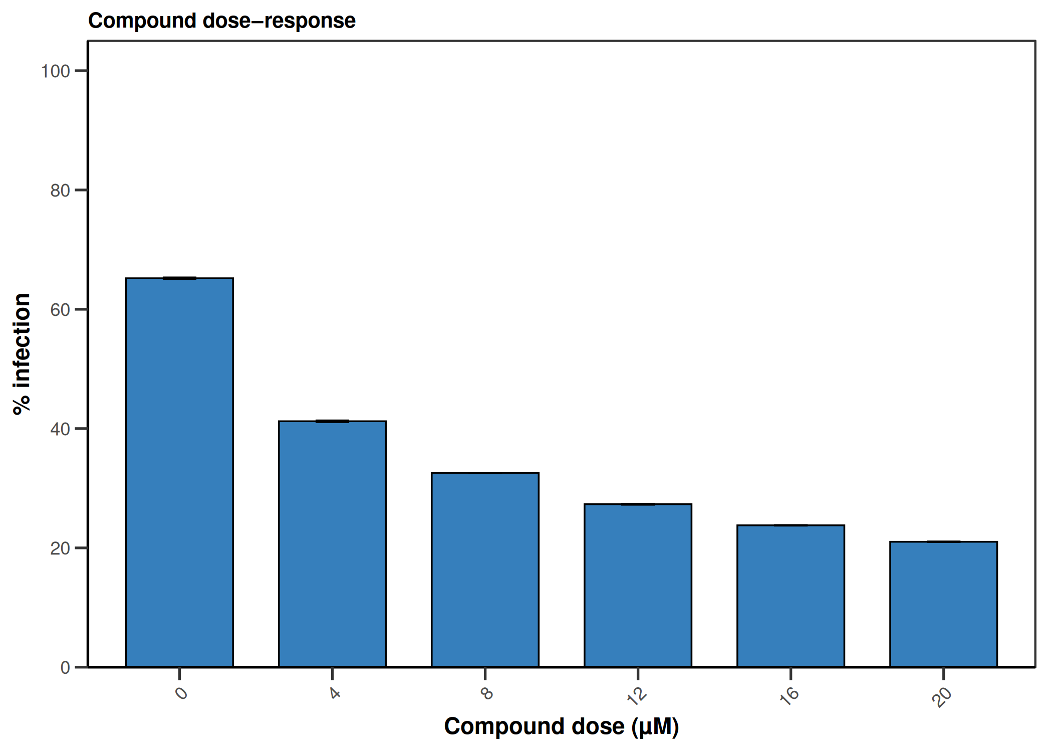
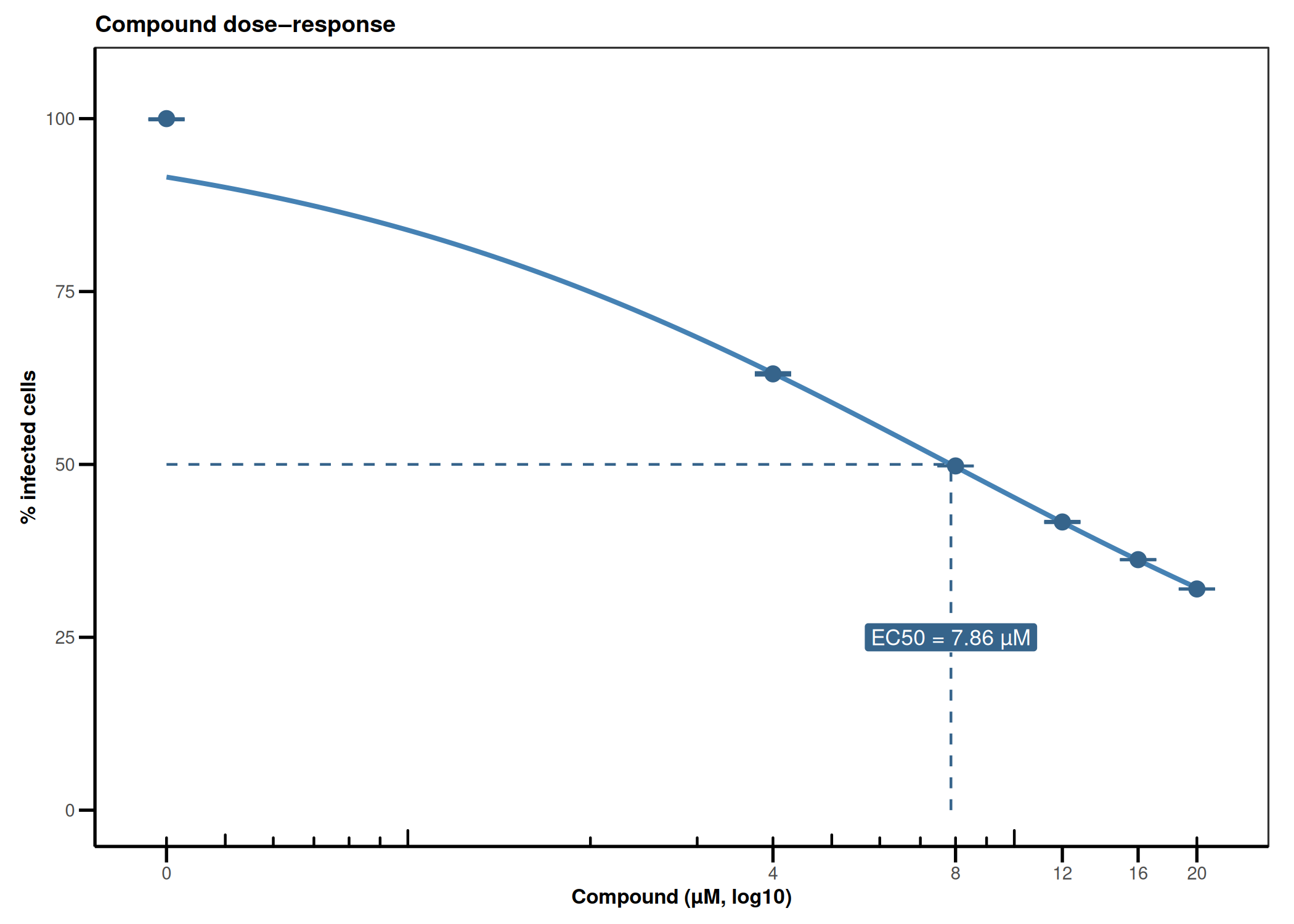
dose-response
microscopy
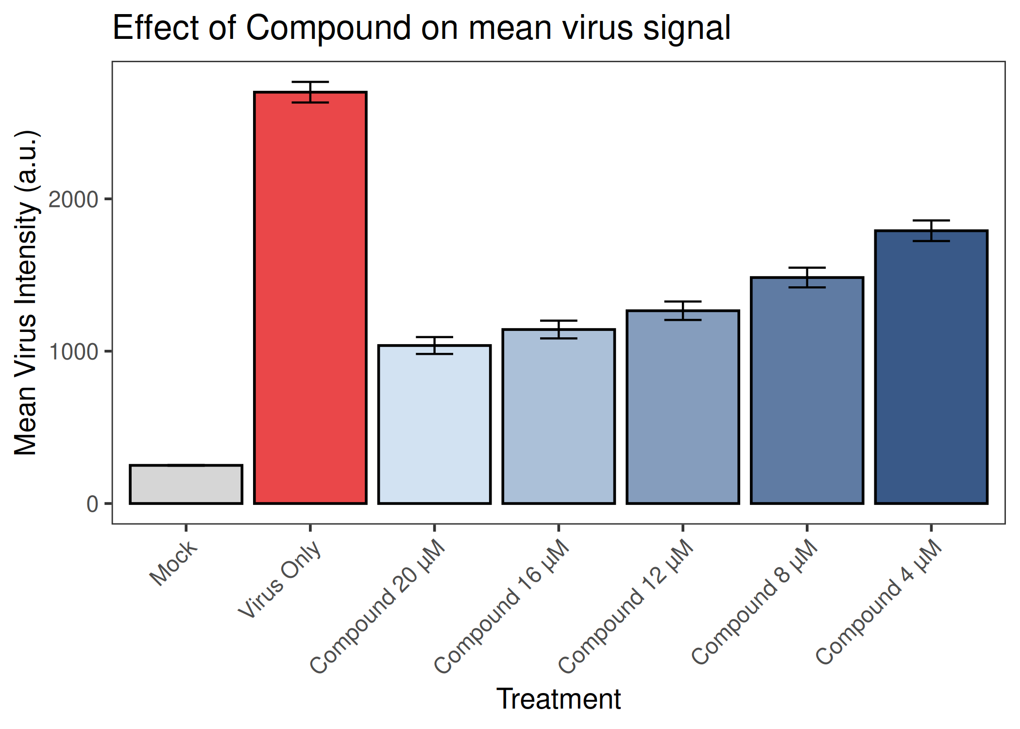
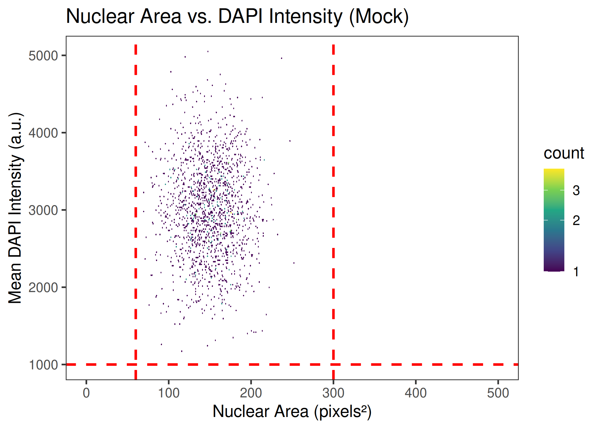
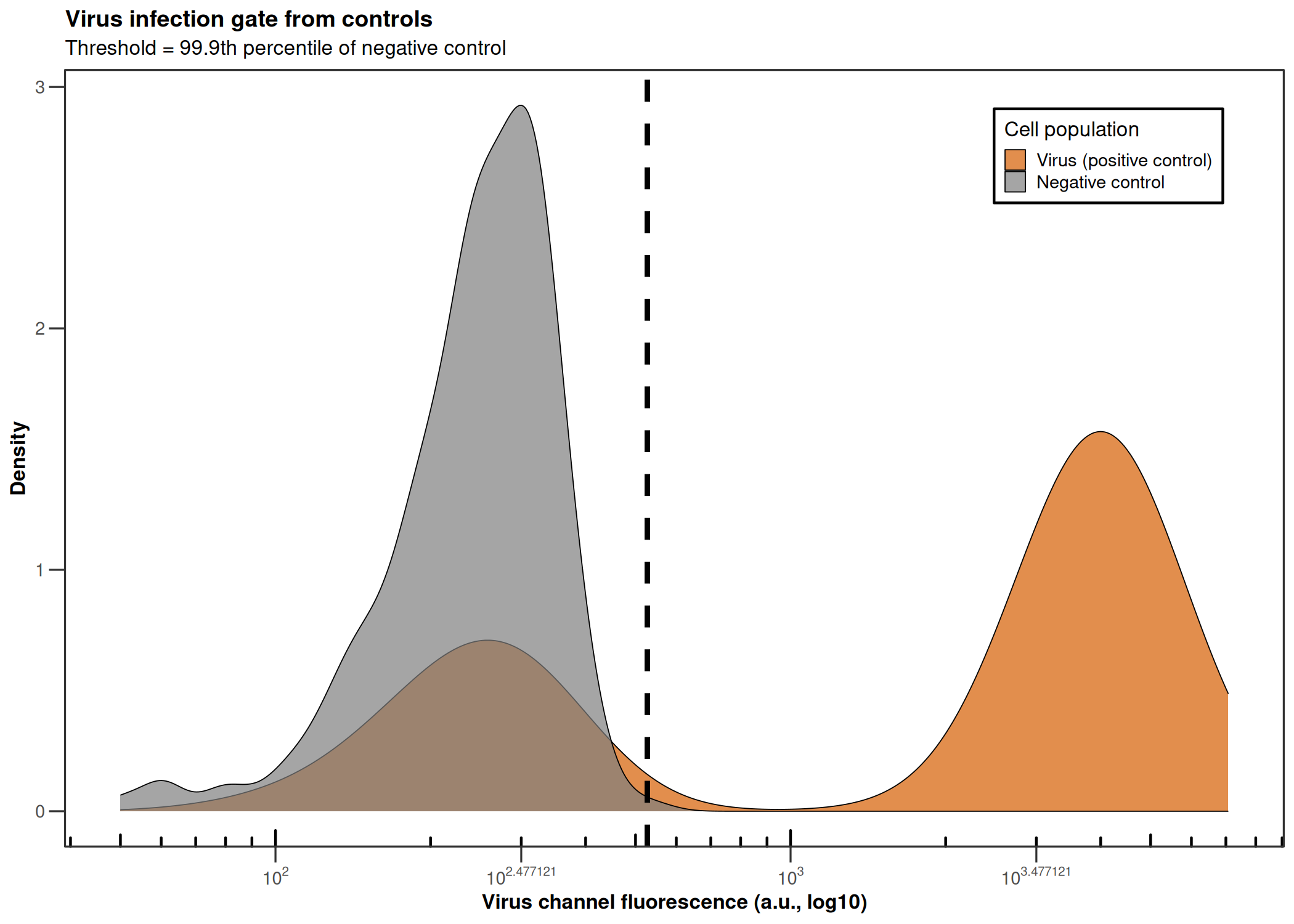
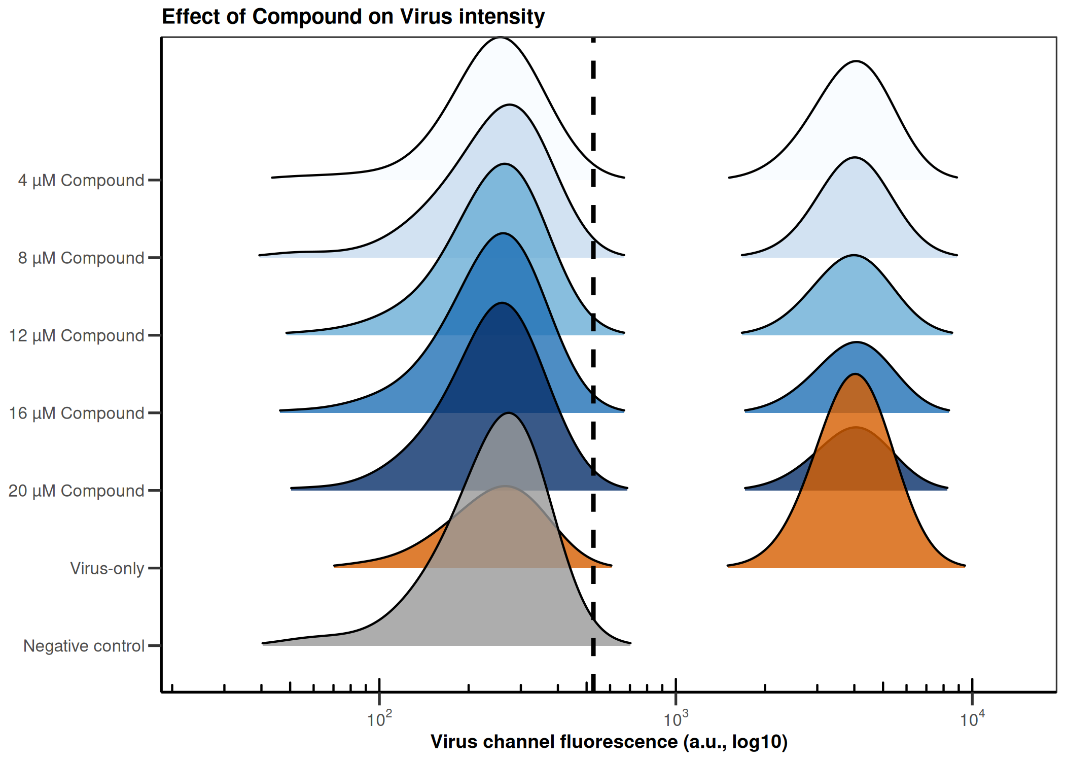
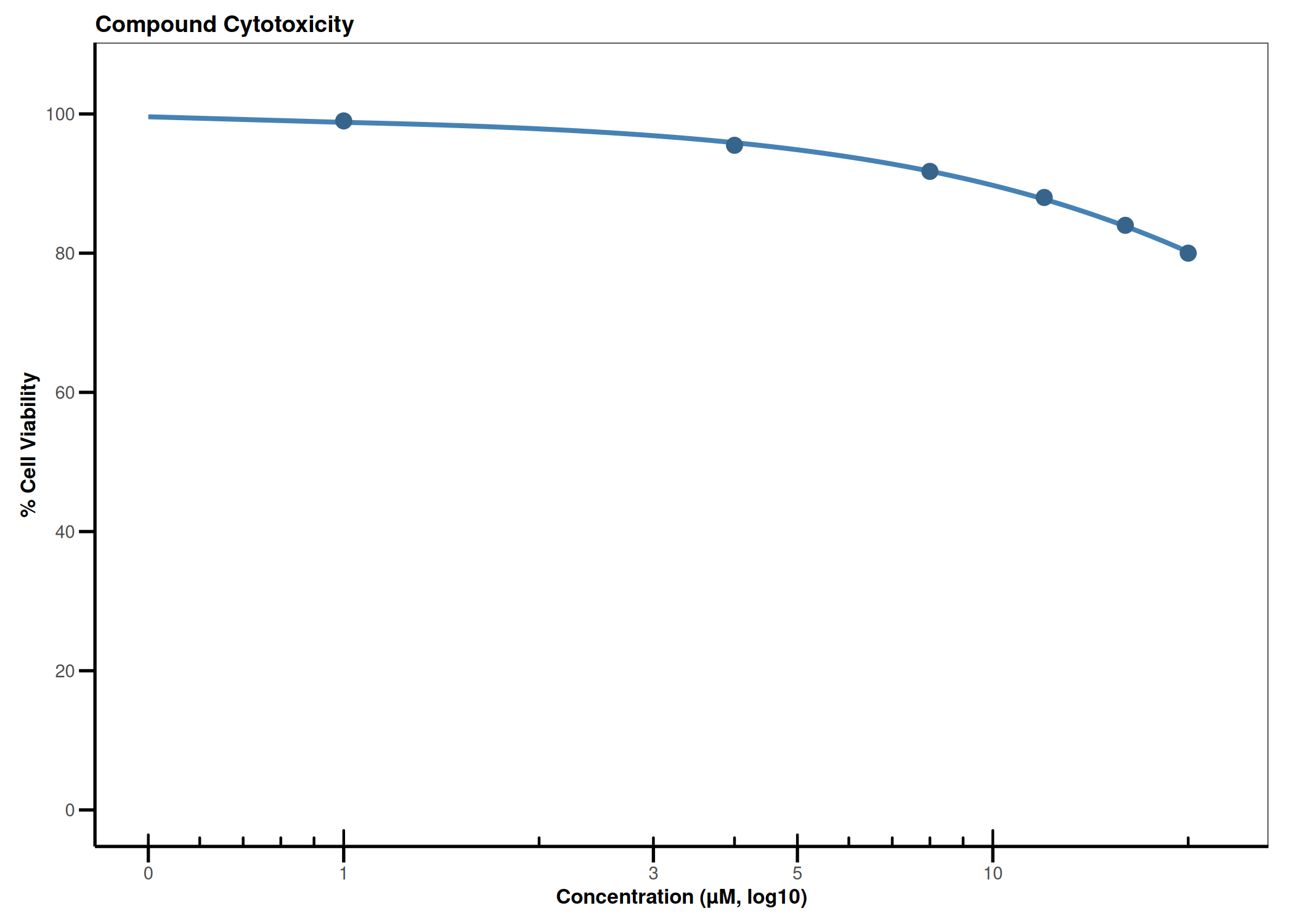
Analyzes per-cell fluorescence data from image-based infection assays (e.g., CQ1 microscope). Gates singlets by nuclear area/DAPI intensity, determines the infection threshold from a negative control, fits a 4PL dose-response model (EC50), fits a cytotoxicity curve (CC50), and computes the Selectivity Index (SI = CC50/EC50).
Overview
Item
Details
Input
Two per-cell CSV files (nucleus channel + virus channel) exported from CQ1 or similar
Key packages
tidyverse, drc, ggridges, scales, ragg
Statistics
4PL dose-response (EC50) · 4PL cytotoxicity (CC50) · Selectivity Index
When to use this template: You have per-cell fluorescence data from a 96-well image-based antiviral assay and want to determine the EC50 of a compound against a viral infection alongside its cytotoxicity.
Note
All plots use Arial 8pt global theme tuned for 4 × 3 inch publication figures. TIFF output at 600 dpi with LZW compression via ragg.
---title: "02 · Image Infection + Dose-Response"subtitle: "CQ1 image-based antiviral assay: gating, EC50, CC50, Selectivity Index"description: | Analyzes per-cell fluorescence data from image-based infection assays (e.g., CQ1 microscope). Gates singlets by nuclear area/DAPI intensity, determines the infection threshold from a negative control, fits a 4PL dose-response model (EC50), fits a cytotoxicity curve (CC50), and computes the Selectivity Index (SI = CC50/EC50).categories: [infection, virology, dose-response, microscopy]---## Overview| Item | Details ||------|---------|| **Input** | Two per-cell CSV files (nucleus channel + virus channel) exported from CQ1 or similar || **Key packages** | `tidyverse`, `drc`, `ggridges`, `scales`, `ragg` || **Statistics** | 4PL dose-response (EC50) · 4PL cytotoxicity (CC50) · Selectivity Index || **Output** | Gating QC · Ridge plot · Bar charts · Dose-response curve · CC50 curve || **Download** | [template.Rmd](template.Rmd) |::: {.callout-tip}**When to use this template:** You have per-cell fluorescence data from a 96-wellimage-based antiviral assay and want to determine the EC50 of a compound against aviral infection alongside its cytotoxicity.:::::: {.callout-note}All plots use **Arial 8pt** global theme tuned for **4 × 3 inch** publication figures.TIFF output at 600 dpi with LZW compression via `ragg`.:::[Back to Gallery](../../index.html){.btn .btn-outline-secondary}[Open Template File](template.Rmd){.btn .btn-primary}```{r child="template.Rmd"}```