10 · RNA-seq TF/Causal Network

Self-contained toy demo: DE-table-first TF activity and causal network exploration

genomics
transcriptomics
RNA-seq
transcription factor
network
demo

A self-contained, offline toy demo of the TF-activity / causal-network workflow. Starts from DESeq2-style contrast tables and scores transcription factors against a small hand-written, CollecTRI-style signed regulon table, checks their overlap with a hand-written, CARNIVAL-style signed prior network, propagates causal sign from a perturbation node, and exports the resulting module networks. Every network is a hardcoded table inside template.Rmd — nothing is downloaded and no solver is run, so the whole thing renders anywhere in seconds.

Overview

Item Details
Input DESeq2-style contrast table: Gene, Comparison, log2FoldChange, padj, optional stat
Key packages dplyr, tidyr, readr, stringr, tibble, igraph, ggplot2, scales
Statistics Hand-rolled signed-regulon TF activity score (sum(mor × de_score) / sqrt(scored targets), direction from the sign of the raw score); prior-network overlap; causal sign propagation from the perturbation node
Output TF volcano/heatmap, TF-to-prior-network diagnostics, recurrent-edge overview, module-specific causal networks, Cytoscape-ready exports (.csv, .sif, .dot)
Download template.Rmd
Important

This is a demo, not a production TF-activity pipeline. The regulon table, the prior knowledge network and the “recurrent CARNIVAL edges” are all small tribble()s written inline in template.Rmd. The template does not call decoupleR, OmnipathR or CARNIVAL, and it does not download anything — that is what keeps it reproducible offline. Its purpose is to demonstrate the shape of the workflow and to give you working plotting, sign-propagation and Cytoscape-export code to hang a real analysis on.

To do the real thing, swap toy_collectri() for a decoupleR regulon (e.g. CollecTRI via OmnipathR), replace the inline pkn tribble with a real signed prior network, and replace the cached carnival_edges with actual CARNIVAL solver output. Those packages are not in install_packages.R precisely because this template never calls them.

Edit the ## ── USER CONFIGURATION block at the top of template.Rmd. Point DEG_FILE at your own DESeq2 contrast table to run the demo statistics over real data; the networks will still be the bundled toy ones until you replace them.

← Gallery Download .Rmd

Code
## ── USER CONFIGURATION ──────────────────────────────────────────────────────
# Input DE table: Gene, Comparison, log2FoldChange, padj, optional stat.
DEG_FILE <- "data/example_deg_results.csv"
GENE_MODULE_FILE <- "data/example_gene_modules.csv"
COMPARISONS_ORDER <- NULL

# DEG / TF filters.
FDR_THRESHOLD <- 0.05
LFC_THRESHOLD <- 1
# Within-contrast |z| a TF must reach to be drawn in a module network. This is a
# *selection* threshold only; the activation/inhibition call comes from the sign
# of the raw activity score, never from the z-score.
TF_ACTIVITY_ABS_CUTOFF <- 0.8
TOP_TF_PER_CONTRAST <- 12
RECURRENT_EDGE_THRESHOLD <- 0.50

# Rebuild the bundled prior networks from the tribbles below instead of reading
# outputs/cache/*.rds. Set TRUE after editing toy_collectri() or the PKN.
FORCE_REFRESH_NETWORK_CACHE <- FALSE

# Optional heavy solver step. This template ships cached toy results and never
# calls CARNIVAL itself; the flags exist so a fork can wire a solver in.
RUN_CARNIVAL_SOLVER <- FALSE
USE_CACHED_CARNIVAL_RESULTS <- TRUE
FORCE_RERUN_SOLVER <- FALSE
SOLVER <- "gurobi"      # gurobi, cplex, cbc, lpSolve

# Plot behavior.
SHOW_RNA_EVIDENCE_BORDER <- TRUE
REMOVE_AMBIGUOUS_NODES_STATIC <- TRUE
RNA_COLOR_LIMIT <- 6
# Fixed seed for the force-directed network layout. Without it every render
# produces different node coordinates and rewrites all 40 PNG/SVG files.
NETWORK_LAYOUT_SEED <- 42
# Font family for figures. "" = the graphics device default, the only portable
# choice: naming a font the device has not registered (e.g. "Arial" on Windows)
# aborts rendering with `invalid font type`.
PLOT_FONT <- ""

OUTPUT_DIR <- "outputs"
## ────────────────────────────────────────────────────────────────────────────

Setup

Code
required_pkgs <- c("dplyr", "tidyr", "readr", "stringr", "tibble", "ggplot2", "scales", "igraph")
missing_pkgs <- required_pkgs[!vapply(required_pkgs, requireNamespace, logical(1), quietly = TRUE)]
if (length(missing_pkgs)) stop("Install required packages: ", paste(missing_pkgs, collapse = ", "))

library(dplyr)
library(tidyr)
library(readr)
library(stringr)
library(tibble)
library(ggplot2)
library(scales)
library(igraph)

paths <- list(
  tables = file.path(OUTPUT_DIR, "tables"),
  plots_overview = file.path(OUTPUT_DIR, "plots", "overview"),
  plots_modules = file.path(OUTPUT_DIR, "plots", "module_networks"),
  source_files = file.path(OUTPUT_DIR, "networks", "source_files"),
  cytoscape = file.path(OUTPUT_DIR, "networks", "cytoscape"),
  cache = file.path(OUTPUT_DIR, "cache")
)
invisible(lapply(paths, dir.create, recursive = TRUE, showWarnings = FALSE))

# The two bundled prior networks are memoised here. FORCE_REFRESH_NETWORK_CACHE
# deletes them so the chunks below genuinely rebuild from the tribbles. The
# CARNIVAL result cache is deliberately NOT touched: that one is governed by
# USE_CACHED_CARNIVAL_RESULTS / FORCE_RERUN_SOLVER.
network_cache_files <- c(
  collectri = file.path(paths$cache, "collectri_signed_tf_target.rds"),
  pkn       = file.path(paths$cache, "omnipath_signed_pkn.rds")
)
if (isTRUE(FORCE_REFRESH_NETWORK_CACHE)) {
  stale <- network_cache_files[file.exists(network_cache_files)]
  if (length(stale)) file.remove(stale)
  message("FORCE_REFRESH_NETWORK_CACHE = TRUE: cleared ", length(stale),
          " cached prior-network file(s) in ", paths$cache)
}

pal <- list(
  predicted_up = "#E08A1E", predicted_down = "#1F5EA8", ambiguous = "#BDBDBD",
  edge_up = "#D97706", edge_down = "#2563A8", edge_unknown = "#8A8A8A",
  rna_down = "#2C7BB6", rna_mid = "#FFFFFF", rna_up = "#B2182B",
  border_rna = "#006D2C", border_default = "#424242"
)

plot_theme <- function(base_size = 10) {
  theme_bw(base_size = base_size, base_family = PLOT_FONT) +
    theme(panel.grid = element_blank(), plot.title = element_text(face = "bold", hjust = 0.5),
          strip.background = element_rect(fill = "grey95", color = "grey70"),
          strip.text = element_text(face = "bold"))
}

Helpers

Code
normalize_gene_symbol <- function(x) {
  x <- stringr::str_trim(as.character(x))
  x <- stringr::str_replace_all(x, "\\s+", "")
  x[x == ""] <- NA_character_
  x
}

safe_name <- function(x) {
  x %>% stringr::str_replace_all("[^A-Za-z0-9]+", "_") %>% stringr::str_replace_all("^_|_$", "")
}

# The bundled toy networks use human-style ALL-CAPS gene symbols. Mouse symbols
# are title case (Ifit1), so case folding is what joins the two. Named rather
# than left as a bare toupper() so the assumption is visible at every call site.
harmonize_symbol <- function(x) toupper(as.character(x))

rna_color <- function(x, limit = RNA_COLOR_LIMIT) {
  x <- pmax(pmin(x, limit), -limit)
  scales::col_numeric(c(pal$rna_down, pal$rna_mid, pal$rna_up), c(-limit, limit))(x)
}

activity_color <- function(x) {
  case_when(is.na(x) ~ pal$ambiguous, x > 0 ~ pal$predicted_up, x < 0 ~ pal$predicted_down, TRUE ~ pal$ambiguous)
}

edge_color <- function(x) {
  case_when(x > 0 ~ pal$edge_up, x < 0 ~ pal$edge_down, TRUE ~ pal$edge_unknown)
}

save_plot_dual <- function(plot, base_path, width = 7, height = 5) {
  png <- paste0(base_path, ".png")
  svg <- paste0(base_path, ".svg")
  ggsave(png, plot, width = width, height = height, units = "in", dpi = 300)
  if (requireNamespace("svglite", quietly = TRUE)) {
    ggsave(svg, plot, width = width, height = height, units = "in", device = svglite::svglite)
  } else {
    message("svglite not installed; skipped SVG: ", svg)
  }
  c(png = png, svg = svg)
}

validate_deg_table <- function(x) {
  required <- c("Gene", "Comparison", "log2FoldChange", "padj")
  missing <- setdiff(required, names(x))
  if (length(missing)) stop("DEG_FILE is missing columns: ", paste(missing, collapse = ", "))
  x %>%
    mutate(Gene = normalize_gene_symbol(Gene), Comparison = as.character(Comparison),
           log2FoldChange = as.numeric(log2FoldChange), padj = as.numeric(padj),
           stat = if ("stat" %in% names(.)) as.numeric(.data$stat) else NA_real_) %>%
    filter(!is.na(Gene), !is.na(Comparison))
}

make_de_score <- function(x) {
  x %>%
    mutate(safe_padj = ifelse(is.na(padj), NA_real_, pmax(padj, .Machine$double.xmin)),
           de_score = ifelse(!is.na(stat), stat, sign(log2FoldChange) * -log10(safe_padj)),
           significant = !is.na(padj) & padj < FDR_THRESHOLD & abs(log2FoldChange) >= LFC_THRESHOLD)
}

Load Data

Code
if (!file.exists(DEG_FILE) || !file.exists(GENE_MODULE_FILE)) {
  source("data/simulate_data.R")
}

deg_all <- read_csv(DEG_FILE, show_col_types = FALSE) %>% validate_deg_table() %>% make_de_score()
if (!is.null(COMPARISONS_ORDER)) {
  deg_all <- deg_all %>% mutate(Comparison = factor(Comparison, levels = COMPARISONS_ORDER))
} else {
  deg_all <- deg_all %>% mutate(Comparison = factor(Comparison, levels = unique(Comparison)))
}

modules <- read_csv(GENE_MODULE_FILE, show_col_types = FALSE) %>%
  transmute(module = as.character(module), gene = normalize_gene_symbol(gene)) %>%
  filter(!is.na(module), !is.na(gene)) %>% distinct()

input_type <- if (all(deg_all$significant)) "significant-DEG-only" else "full-DE-results"
cat("DE input type:", input_type, "\n")
DE input type: full-DE-results 
Code
cat("Genes:", n_distinct(deg_all$Gene), "\n")
Genes: 51 
Code
cat("Comparisons:", paste(levels(deg_all$Comparison), collapse = ", "), "\n")
Comparisons: Treatment_24h_vs_Control, Treatment_48h_vs_Control, Recovery_96h_vs_Control 
Code
cat("Significant DE rows:", sum(deg_all$significant), "\n")
Significant DE rows: 31 
Code
write_csv(deg_all, file.path(paths$tables, "validated_deg_results.csv"))
write_csv(modules, file.path(paths$tables, "gene_modules.csv"))

Signed CollecTRI-Style TF-Target Network

A hand-written 36-row signed regulon table in the shape CollecTRI uses (tf, target, mor = mode of regulation). This is not CollecTRI and this template does not call decoupleR or OmnipathR — keeping the network inline is what lets the whole document render offline. To use a real regulon, return one from toy_collectri() with the same three columns.

Code
toy_collectri <- function() {
  tribble(
    ~tf, ~target, ~mor,
    "STAT1", "IFIT1", 1, "STAT1", "ISG15", 1, "STAT1", "CXCL10", 1, "STAT1", "IRF7", 1,
    "IRF1", "IFIT1", 1, "IRF1", "CXCL10", 1, "IRF1", "ICAM1", 1,
    "IRF7", "ISG15", 1, "IRF7", "MX1", 1, "IRF7", "OAS1", 1,
    "NFKB1", "ICAM1", 1, "NFKB1", "VCAM1", 1, "NFKB1", "CCL2", 1, "NFKB1", "PTGS2", 1,
    "RELA", "ICAM1", 1, "RELA", "CXCL10", 1, "RELA", "TNF", 1, "RELA", "MMP3", 1,
    "JUN", "MMP3", 1, "JUN", "PTGS2", 1, "JUN", "VEGFA", 1,
    "FOS", "MMP3", 1, "FOS", "PTGS2", 1, "FOS", "VEGFA", 1,
    "HIF1A", "VEGFA", 1, "HIF1A", "NOS2", 1, "HIF1A", "ANGPT2", 1,
    "SPI1", "ITGAM", 1, "SPI1", "LYZ2", 1, "SPI1", "S100A9", 1,
    "ETS1", "VCAM1", 1, "ETS1", "MMP9", 1, "ETS1", "COL4A1", -1,
    "KLF2", "ICAM1", -1, "KLF2", "VCAM1", -1, "KLF2", "THBD", 1
  )
}

collectri_cache <- network_cache_files[["collectri"]]
if (file.exists(collectri_cache)) {
  collectri <- readRDS(collectri_cache)
} else {
  collectri <- toy_collectri()
  saveRDS(collectri, collectri_cache)
}
write_csv(collectri, file.path(paths$tables, "collectri_tf_target_network.csv"))

TF Activity

Code
tf_activity <- deg_all %>%
  mutate(target = harmonize_symbol(Gene)) %>%
  # Many-to-many is expected: one gene appears once per contrast on the left and
  # can be regulated by several TFs on the right.
  inner_join(collectri, by = "target", relationship = "many-to-many") %>%
  group_by(Comparison, tf) %>%
  summarise(
    # Mean-of-signed-scores scaled by sqrt(n): divide by the number of targets
    # that actually contributed a score, not by n(), which counts NA rows too
    # and silently dilutes the activity of regulons with missing DE values.
    scored_targets = sum(!is.na(mor * de_score)),
    activity = if (scored_targets > 0) {
      sum(mor * de_score, na.rm = TRUE) / sqrt(scored_targets)
    } else {
      NA_real_
    },
    target_count = n_distinct(target),
    .groups = "drop"
  ) %>%
  group_by(Comparison) %>%
  # activity_z ranks TFs *within* a contrast; it is a relative measure and says
  # nothing about direction (a z below the contrast mean can still be a positive
  # activity). Direction therefore comes from sign(activity), never from the z.
  mutate(activity_z = as.numeric(scale(activity)),
         predicted_state = case_when(is.na(activity) ~ "ambiguous",
                                     sign(activity) > 0 ~ "predicted activation",
                                     sign(activity) < 0 ~ "predicted inhibition",
                                     TRUE ~ "ambiguous")) %>%
  ungroup() %>%
  arrange(Comparison, desc(abs(activity_z)))

write_csv(tf_activity, file.path(paths$tables, "tf_activity_scores.csv"))
tf_activity %>%
  group_by(Comparison) %>%
  slice_max(abs(activity_z), n = 5) %>%
  ungroup() %>%
  select(Comparison, tf, activity, target_count, scored_targets, activity_z, predicted_state) %>%
  knitr::kable(
    caption   = "Top 5 Inferred Transcription Factors per Comparison",
    col.names = c("Comparison", "TF", "Activity Score", "Target Count", "Scored Targets",
                  "Within-contrast z (ranking only)", "Predicted State"),
    digits    = 3
  )
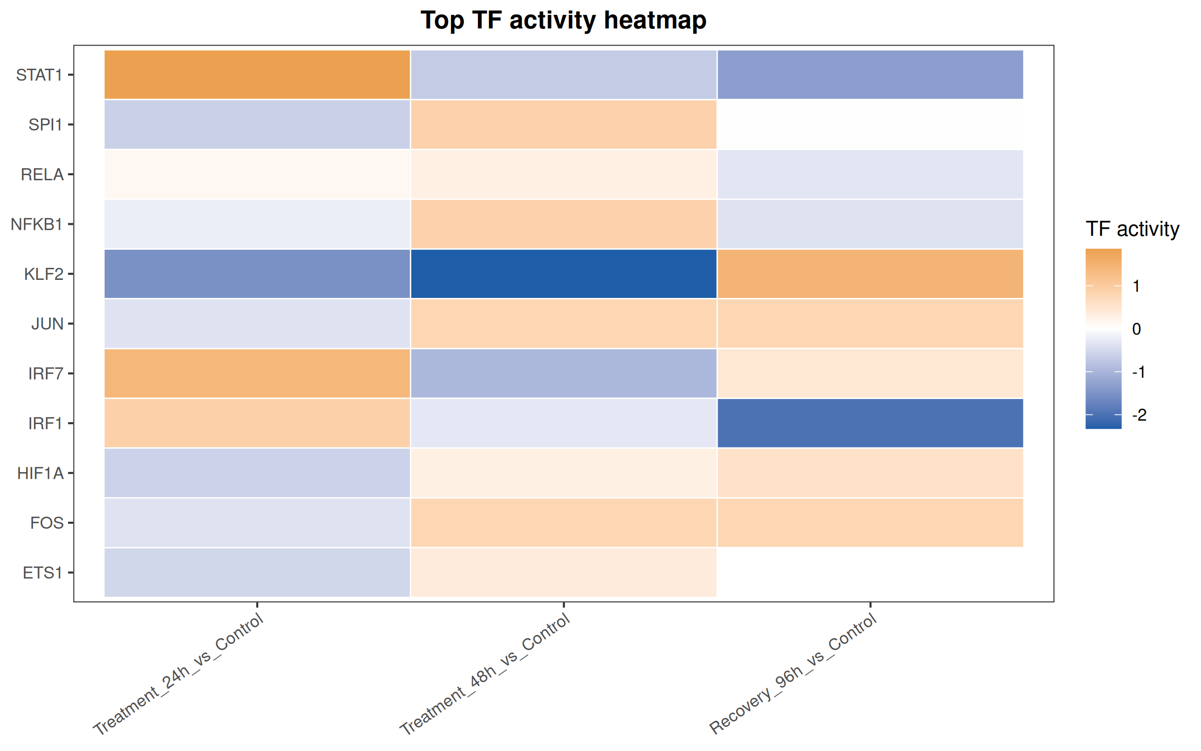
Top 5 Inferred Transcription Factors per Comparison
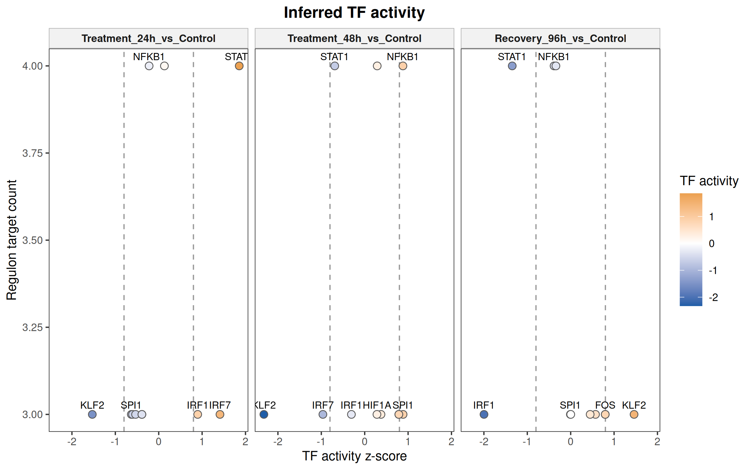
Comparison TF Activity Score Target Count Scored Targets Within-contrast z (ranking only) Predicted State
Treatment_24h_vs_Control STAT1 12.415 4 4 1.856 predicted activation
Treatment_24h_vs_Control KLF2 -5.541 3 3 -1.531 predicted inhibition
Treatment_24h_vs_Control IRF7 10.061 3 3 1.412 predicted activation
Treatment_24h_vs_Control IRF1 7.338 3 3 0.898 predicted activation
Treatment_24h_vs_Control SPI1 -0.775 3 3 -0.632 predicted inhibition
Treatment_48h_vs_Control KLF2 -12.097 3 3 -2.324 predicted inhibition
Treatment_48h_vs_Control IRF7 -1.747 3 3 -0.964 predicted inhibition
Treatment_48h_vs_Control SPI1 12.313 3 3 0.884 predicted activation
Treatment_48h_vs_Control NFKB1 12.285 4 4 0.881 predicted activation
Treatment_48h_vs_Control FOS 11.570 3 3 0.787 predicted activation
Treatment_48h_vs_Control JUN 11.570 3 3 0.787 predicted activation
Recovery_96h_vs_Control IRF1 -10.526 3 3 -1.998 predicted inhibition
Recovery_96h_vs_Control KLF2 6.688 3 3 1.461 predicted activation
Recovery_96h_vs_Control STAT1 -7.287 4 4 -1.347 predicted inhibition
Recovery_96h_vs_Control FOS 3.381 3 3 0.796 predicted activation
Recovery_96h_vs_Control JUN 3.381 3 3 0.796 predicted activation

Signed OmniPath-Style PKN And TF Overlap

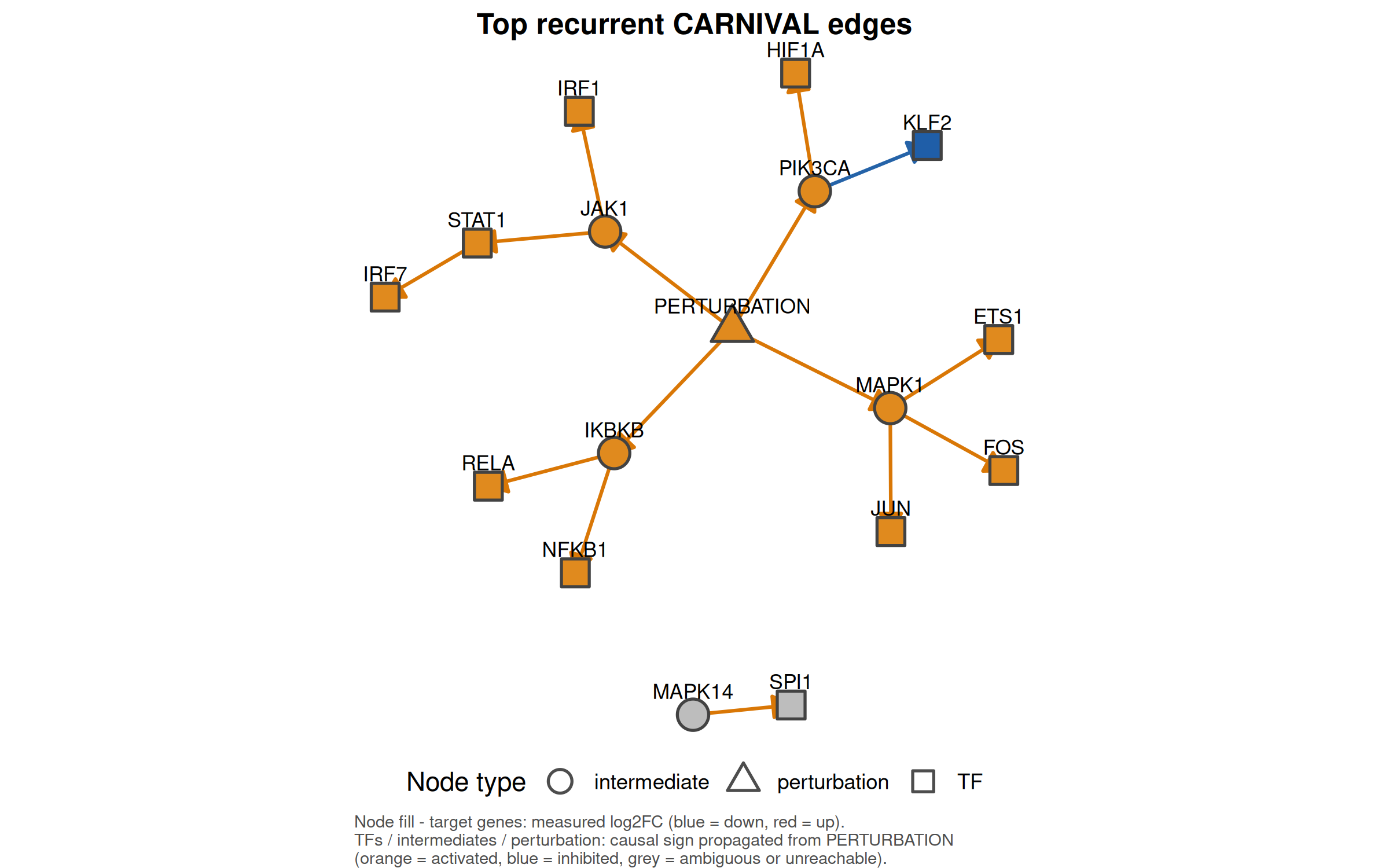
Likewise a hand-written 15-edge signed prior knowledge network in OmniPath’s source / target / sign shape, rooted at a synthetic PERTURBATION node. Replace the tribble() with a real signed PKN to use this on live data.

Code
pkn_cache <- network_cache_files[["pkn"]]
if (file.exists(pkn_cache)) {
  pkn <- readRDS(pkn_cache)
} else {
  pkn <- tribble(
    ~source, ~target, ~sign,
    "PERTURBATION", "MAPK1", 1, "PERTURBATION", "IKBKB", 1, "PERTURBATION", "JAK1", 1,
    "PERTURBATION", "PIK3CA", 1, "MAPK1", "JUN", 1, "MAPK1", "FOS", 1,
    "IKBKB", "NFKB1", 1, "IKBKB", "RELA", 1, "JAK1", "STAT1", 1, "JAK1", "IRF1", 1,
    "STAT1", "IRF7", 1, "PIK3CA", "HIF1A", 1, "PIK3CA", "KLF2", -1,
    "MAPK1", "ETS1", 1, "MAPK14", "SPI1", 1
  )
  saveRDS(pkn, pkn_cache)
}
write_csv(pkn, file.path(paths$tables, "omnipath_signed_pkn.csv"))
pkn_nodes <- unique(c(pkn$source, pkn$target))

tf_pkn_overlap <- tf_activity %>%
  mutate(in_pkn = tf %in% pkn_nodes) %>%
  group_by(Comparison) %>%
  summarise(tf_total = n_distinct(tf), tf_in_pkn = n_distinct(tf[in_pkn]),
            tf_not_in_pkn = tf_total - tf_in_pkn, overlap_fraction = tf_in_pkn / tf_total, .groups = "drop")
write_csv(tf_pkn_overlap, file.path(paths$tables, "tf_to_pkn_overlap.csv"))

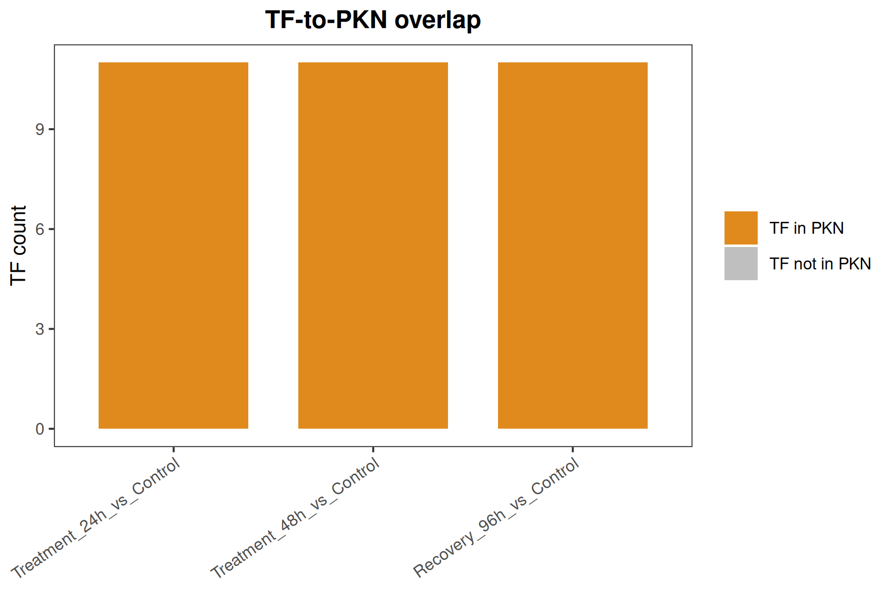
p_overlap <- tf_pkn_overlap %>%
  pivot_longer(c(tf_in_pkn, tf_not_in_pkn), names_to = "class", values_to = "n") %>%
  mutate(class = recode(class, tf_in_pkn = "TF in PKN", tf_not_in_pkn = "TF not in PKN")) %>%
  ggplot(aes(Comparison, n, fill = class)) +
  geom_col(width = 0.75) +
  scale_fill_manual(values = c("TF in PKN" = pal$predicted_up, "TF not in PKN" = "grey75")) +
  labs(x = NULL, y = "TF count", fill = NULL, title = "TF-to-PKN overlap") +
  plot_theme() + theme(axis.text.x = element_text(angle = 35, hjust = 1))
save_plot_dual(p_overlap, file.path(paths$plots_overview, "tf_to_pkn_overlap"), 6, 4)
                                           png 
"outputs/plots/overview/tf_to_pkn_overlap.png" 
                                           svg 
"outputs/plots/overview/tf_to_pkn_overlap.svg" 
Code
p_overlap

Cached CARNIVAL-Style Results

No solver is run here and CARNIVAL is never called. The “recurrent edges” below are the same 15 hand-written PKN edges with invented recurrence weights, in the shape CARNIVAL’s per-sample solutions would have after aggregation. The RUN_CARNIVAL_SOLVER / SOLVER knobs and the solver_available() probe exist so a fork can drop a real solver call in at this point.

Code
solver_available <- function(solver) {
  solver <- tolower(solver)
  switch(solver,
    gurobi = nzchar(Sys.which("gurobi_cl")) || requireNamespace("gurobi", quietly = TRUE),
    cplex = nzchar(Sys.which("cplex")) || requireNamespace("Rcplex", quietly = TRUE),
    cbc = nzchar(Sys.which("cbc")) || nzchar(Sys.which("cbc.exe")),
    lpsolve = requireNamespace("lpSolve", quietly = TRUE), FALSE)
}
if (RUN_CARNIVAL_SOLVER && (!requireNamespace("CARNIVAL", quietly = TRUE) || !solver_available(SOLVER))) {
  message("CARNIVAL or solver not available; using cached/demo results.")
}

carnival_cache <- file.path(paths$cache, "cached_carnival_recurrent_edges.rds")
if (file.exists(carnival_cache) && USE_CACHED_CARNIVAL_RESULTS && !FORCE_RERUN_SOLVER) {
  carnival_edges <- readRDS(carnival_cache)
} else {
  base_edges <- tribble(
    ~source, ~target, ~sign, ~recurrence,
    "PERTURBATION", "MAPK1", 1, 1.00, "PERTURBATION", "IKBKB", 1, 0.85,
    "PERTURBATION", "JAK1", 1, 0.80, "PERTURBATION", "PIK3CA", 1, 0.65,
    "MAPK1", "JUN", 1, 0.90, "MAPK1", "FOS", 1, 0.75,
    "IKBKB", "NFKB1", 1, 0.88, "IKBKB", "RELA", 1, 0.82,
    "JAK1", "STAT1", 1, 0.95, "JAK1", "IRF1", 1, 0.70,
    "STAT1", "IRF7", 1, 0.62, "PIK3CA", "HIF1A", 1, 0.72,
    "PIK3CA", "KLF2", -1, 0.55, "MAPK1", "ETS1", 1, 0.58,
    "MAPK14", "SPI1", 1, 0.52
  )
  carnival_edges <- bind_rows(lapply(levels(deg_all$Comparison), function(comp) mutate(base_edges, Comparison = comp)))
  saveRDS(carnival_edges, carnival_cache)
}
carnival_edges <- carnival_edges %>% filter(recurrence >= RECURRENT_EDGE_THRESHOLD)
write_csv(carnival_edges, file.path(paths$tables, "carnival_recurrent_edges.csv"))

Overview Plots

Code
top_tfs <- tf_activity %>% group_by(Comparison) %>% slice_max(abs(activity_z), n = TOP_TF_PER_CONTRAST, with_ties = FALSE) %>% ungroup()

p_tf <- tf_activity %>%
  ggplot(aes(activity_z, target_count)) +
  geom_vline(xintercept = c(-TF_ACTIVITY_ABS_CUTOFF, TF_ACTIVITY_ABS_CUTOFF), linetype = "dashed", color = "grey60") +
  geom_point(aes(fill = activity_z), shape = 21, color = "grey35", size = 2.5) +
  geom_text(data = top_tfs, aes(label = tf), size = 2.7, vjust = -0.8, check_overlap = TRUE) +
  facet_wrap(~Comparison) +
  scale_fill_gradient2(low = pal$predicted_down, mid = "white", high = pal$predicted_up, midpoint = 0, name = "TF activity") +
  labs(x = "TF activity z-score", y = "Regulon target count", title = "Inferred TF activity") + plot_theme()
save_plot_dual(p_tf, file.path(paths$plots_overview, "tf_activity_volcano"), 8, 5)
                                             png 
"outputs/plots/overview/tf_activity_volcano.png" 
                                             svg 
"outputs/plots/overview/tf_activity_volcano.svg" 
Code
p_tf

Code
p_heat <- tf_activity %>%
  semi_join(top_tfs %>% distinct(tf), by = "tf") %>%
  ggplot(aes(Comparison, tf, fill = activity_z)) +
  geom_tile(color = "white", linewidth = 0.3) +
  scale_fill_gradient2(low = pal$predicted_down, mid = "white", high = pal$predicted_up, midpoint = 0, name = "TF activity") +
  labs(x = NULL, y = NULL, title = "Top TF activity heatmap") + plot_theme() +
  theme(axis.text.x = element_text(angle = 35, hjust = 1))
save_plot_dual(p_heat, file.path(paths$plots_overview, "tf_activity_heatmap"), 6, 5)
                                             png 
"outputs/plots/overview/tf_activity_heatmap.png" 
                                             svg 
"outputs/plots/overview/tf_activity_heatmap.svg" 
Code
p_heat

Network Helpers

Code
# Causal sign propagation.
#
# Start the perturbation at +1 and push the sign forward along DIRECTED edges:
# a node's state is its upstream state multiplied by the edge sign. A node
# reached with two conflicting signs is ambiguous (0); a node not reachable from
# the perturbation at all is unknown (NA). Both render grey.
#
# This replaces an earlier version that summed a node's incoming AND outgoing
# edge signs. That is not sign propagation - it is a degree statistic - and in a
# predominantly activating prior network it made almost every node come out +1.
propagate_sign_from_perturbation <- function(edges, root = "PERTURBATION") {
  nodes <- sort(unique(c(edges$source, edges$target)))
  state <- setNames(rep(NA_real_, length(nodes)), nodes)

  if (!root %in% nodes) {
    return(tibble(node = nodes, predicted_activity = NA_real_))
  }
  state[[root]] <- 1

  e <- edges %>%
    filter(!is.na(sign)) %>%
    distinct(source, target, sign) %>%
    mutate(sign = sign(sign))

  # State only ever moves NA -> +/-1 -> 0, and 0 is absorbing, so this converges
  # in at most one pass per node even when the graph contains cycles.
  for (iter in seq_along(nodes)) {
    changed <- FALSE
    for (i in seq_len(nrow(e))) {
      upstream <- state[[e$source[[i]]]]
      if (is.na(upstream)) next
      proposed <- upstream * e$sign[[i]]
      current  <- state[[e$target[[i]]]]
      updated  <- if (is.na(current)) proposed else if (current == proposed) current else 0
      if (is.na(current) || current != updated) {
        state[[e$target[[i]]]] <- updated
        changed <- TRUE
      }
    }
    if (!changed) break
  }

  tibble(node = names(state), predicted_activity = unname(state))
}

upstream_closure <- function(edges, seeds) {
  selected <- edges[0, ]; frontier <- unique(seeds); visited_edges <- character()
  repeat {
    hit <- edges %>% filter(target %in% frontier, !(paste(source, target) %in% visited_edges))
    if (!nrow(hit)) break
    selected <- bind_rows(selected, hit) %>% distinct()
    visited_edges <- unique(c(visited_edges, paste(hit$source, hit$target)))
    frontier <- setdiff(unique(hit$source), unique(c(seeds, selected$target)))
    if (!length(frontier)) break
  }
  selected
}

write_network_sidecars <- function(edges, nodes, out_prefix) {
  dir.create(dirname(out_prefix), recursive = TRUE, showWarnings = FALSE)
  write_tsv(edges %>% transmute(source, interaction = ifelse(sign > 0, "activates", ifelse(sign < 0, "inhibits", "interacts")), target),
            paste0(out_prefix, ".sif"), col_names = FALSE)
  write_csv(nodes, paste0(out_prefix, "_node_attributes.csv"))
  write_csv(edges, paste0(out_prefix, "_edge_attributes.csv"))
  dot_nodes <- nodes %>% mutate(shape_dot = case_when(node_type == "TF" ~ "box", node_type == "perturbation" ~ "plaintext", TRUE ~ "ellipse")) %>%
    transmute(line = paste0('  "', node, '" [label="', node, '", shape=', shape_dot, ', style=filled, fillcolor="', fill_color, '", color="', border_color, '"];'))
  dot_edges <- edges %>% transmute(line = paste0('  "', source, '" -> "', target, '" [color="', edge_color(sign), '"];'))
  # Helvetica is one of Graphviz's built-in PostScript font names, so the .dot
  # renders identically everywhere; "Arial" resolves only where it is installed.
  writeLines(c("digraph causal_network {", "  graph [rankdir=LR, fontname=Helvetica];", "  node [fontname=Helvetica];", "  edge [fontname=Helvetica];", dot_nodes$line, dot_edges$line, "}"), paste0(out_prefix, ".dot"))
}

plot_network <- function(edges, nodes, title) {
  if (!nrow(edges) || !nrow(nodes)) return(ggplot() + annotate("text", 0, 0, label = "No network edges after filtering") + theme_void())
  graph <- graph_from_data_frame(edges %>% select(source, target), directed = TRUE, vertices = nodes %>% select(node))
  # layout_with_fr() is stochastic. Without a fixed seed every render produces new
  # coordinates and rewrites every PNG/SVG, which is permanent binary churn in git.
  set.seed(NETWORK_LAYOUT_SEED)
  coords <- as_tibble(layout_with_fr(graph), .name_repair = "minimal") %>% setNames(c("x", "y")) %>% mutate(node = V(graph)$name) %>% left_join(nodes, by = "node")
  edge_xy <- edges %>%
    left_join(coords %>% select(node, x_source = x, y_source = y), by = c("source" = "node")) %>%
    left_join(coords %>% select(node, x_target = x, y_target = y), by = c("target" = "node"))
  ggplot() +
    geom_segment(data = edge_xy, aes(x = x_source, y = y_source, xend = x_target, yend = y_target, color = edge_color(sign)), linewidth = 0.7,
                 arrow = grid::arrow(length = grid::unit(0.12, "inches"), type = "closed"), lineend = "round") +
    geom_point(data = coords, aes(x, y, shape = node_type, fill = fill_color, color = border_color), size = 5.5, stroke = 0.9) +
    geom_text(data = coords, aes(x, y, label = node), size = 3, family = PLOT_FONT, vjust = -1.05, check_overlap = TRUE) +
    scale_shape_manual(values = c(TF = 22, gene = 21, intermediate = 21, perturbation = 24), drop = FALSE) +
    scale_fill_identity() + scale_color_identity() +
    guides(shape = guide_legend(title = "Node type", override.aes = list(fill = "white", color = "grey30", size = 4))) +
    labs(
      title = title,
      # The fill channel carries two different things, so say which is which.
      caption = paste(
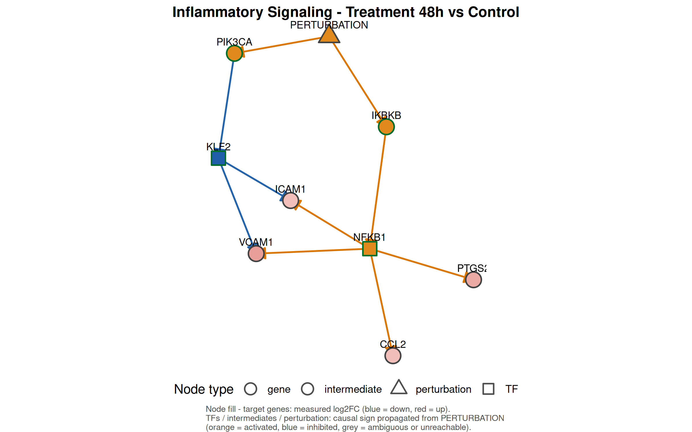
        "Node fill - target genes: measured log2FC (blue = down, red = up).",
        "TFs / intermediates / perturbation: causal sign propagated from PERTURBATION",
        "(orange = activated, blue = inhibited, grey = ambiguous or unreachable).",
        sep = "\n"
      )
    ) +
    coord_equal() + theme_void(base_family = PLOT_FONT) +
    theme(plot.title = element_text(face = "bold", hjust = 0.5, size = 12),
          plot.caption = element_text(hjust = 0, size = 7, color = "grey30"),
          legend.position = "bottom")
}

build_module_network <- function(comparison_name, module_name) {
  sig_targets <- deg_all %>% filter(as.character(Comparison) == comparison_name, significant) %>% mutate(target = harmonize_symbol(Gene)) %>% inner_join(modules %>% mutate(target = harmonize_symbol(gene)), by = "target") %>% filter(module == module_name)
  if (!nrow(sig_targets)) return(NULL)
  active_tfs <- tf_activity %>% filter(as.character(Comparison) == comparison_name, abs(activity_z) >= TF_ACTIVITY_ABS_CUTOFF) %>% pull(tf)
  tf_edges <- collectri %>% semi_join(sig_targets, by = "target") %>% filter(tf %in% active_tfs) %>% transmute(source = tf, target, sign = mor, recurrence = 1, edge_class = "TF-target")
  if (!nrow(tf_edges)) return(NULL)
  upstream_edges <- carnival_edges %>% filter(as.character(Comparison) == comparison_name) %>% select(source, target, sign, recurrence) %>% mutate(edge_class = "CARNIVAL-PKN") %>% upstream_closure(unique(tf_edges$source))
  edges <- bind_rows(upstream_edges, tf_edges) %>% distinct(source, target, .keep_all = TRUE)
  pred <- propagate_sign_from_perturbation(edges)
  rna_here <- deg_all %>% filter(as.character(Comparison) == comparison_name) %>% mutate(node = harmonize_symbol(Gene))
  nodes <- tibble(node = sort(unique(c(edges$source, edges$target)))) %>%
    mutate(node_type = case_when(node == "PERTURBATION" ~ "perturbation", node %in% unique(tf_edges$source) ~ "TF", node %in% unique(tf_edges$target) ~ "gene", TRUE ~ "intermediate")) %>%
    left_join(pred, by = "node") %>% left_join(rna_here %>% select(node, log2FoldChange, padj, significant), by = "node") %>%
    mutate(fill_color = ifelse(node_type == "gene" & !is.na(log2FoldChange), rna_color(log2FoldChange), activity_color(predicted_activity)),
           border_color = ifelse(SHOW_RNA_EVIDENCE_BORDER & node_type != "gene" & !is.na(log2FoldChange), pal$border_rna, pal$border_default))
  if (REMOVE_AMBIGUOUS_NODES_STATIC) {
    keep <- nodes %>% filter(node_type %in% c("perturbation", "gene") | (!is.na(predicted_activity) & predicted_activity != 0)) %>% pull(node)
    edges <- edges %>% filter(source %in% keep, target %in% keep)
    nodes <- nodes %>% filter(node %in% unique(c(edges$source, edges$target)))
  }
  list(edges = edges, nodes = nodes, targets = unique(sig_targets$Gene), tfs = unique(tf_edges$source))
}
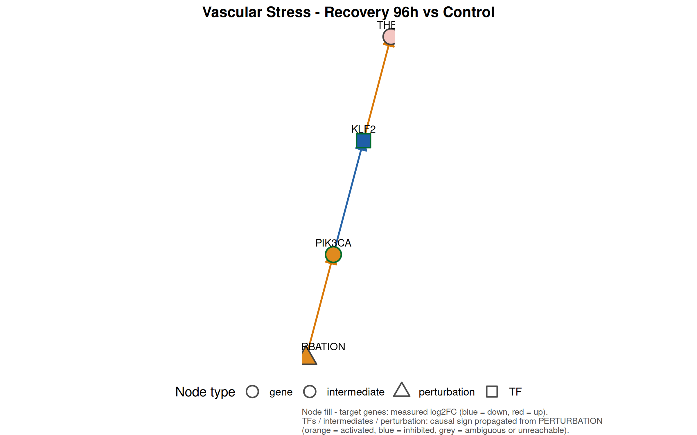
Network Figures And Exports

Code
overview_edges <- carnival_edges %>% group_by(source, target, sign) %>% summarise(recurrence = mean(recurrence), edge_class = "CARNIVAL-PKN", .groups = "drop")
overview_nodes <- tibble(node = sort(unique(c(overview_edges$source, overview_edges$target)))) %>% left_join(propagate_sign_from_perturbation(overview_edges), by = "node") %>% mutate(node_type = case_when(node == "PERTURBATION" ~ "perturbation", node %in% unique(tf_activity$tf) ~ "TF", TRUE ~ "intermediate"), fill_color = activity_color(predicted_activity), border_color = pal$border_default)
write_network_sidecars(overview_edges, overview_nodes, file.path(paths$source_files, "recurrent_edge_overview"))
write_csv(overview_edges, file.path(paths$cytoscape, "recurrent_edge_overview_edges.csv"))
write_csv(overview_nodes, file.path(paths$cytoscape, "recurrent_edge_overview_nodes.csv"))
p_overview <- plot_network(overview_edges, overview_nodes, "Top recurrent CARNIVAL edges")
save_plot_dual(p_overview, file.path(paths$plots_overview, "top_recurrent_edges"), 8, 5)
                                             png 
"outputs/plots/overview/top_recurrent_edges.png" 
                                             svg 
"outputs/plots/overview/top_recurrent_edges.svg" 
Code
p_overview

Code
module_summary <- list()
for (comp in levels(deg_all$Comparison)) {
  comp_dir <- file.path(paths$plots_modules, safe_name(comp)); src_dir <- file.path(paths$source_files, "module_networks", safe_name(comp)); cy_dir <- file.path(paths$cytoscape, "module_networks", safe_name(comp))
  dir.create(comp_dir, recursive = TRUE, showWarnings = FALSE); dir.create(src_dir, recursive = TRUE, showWarnings = FALSE); dir.create(cy_dir, recursive = TRUE, showWarnings = FALSE)
  for (mod in unique(modules$module)) {
    net <- build_module_network(comp, mod)
    if (is.null(net)) next
    base <- safe_name(mod); sidecar_prefix <- file.path(src_dir, base)
    write_network_sidecars(net$edges, net$nodes, sidecar_prefix)
    write_csv(net$edges, file.path(cy_dir, paste0(base, "_edges.csv"))); write_csv(net$nodes, file.path(cy_dir, paste0(base, "_nodes.csv")))
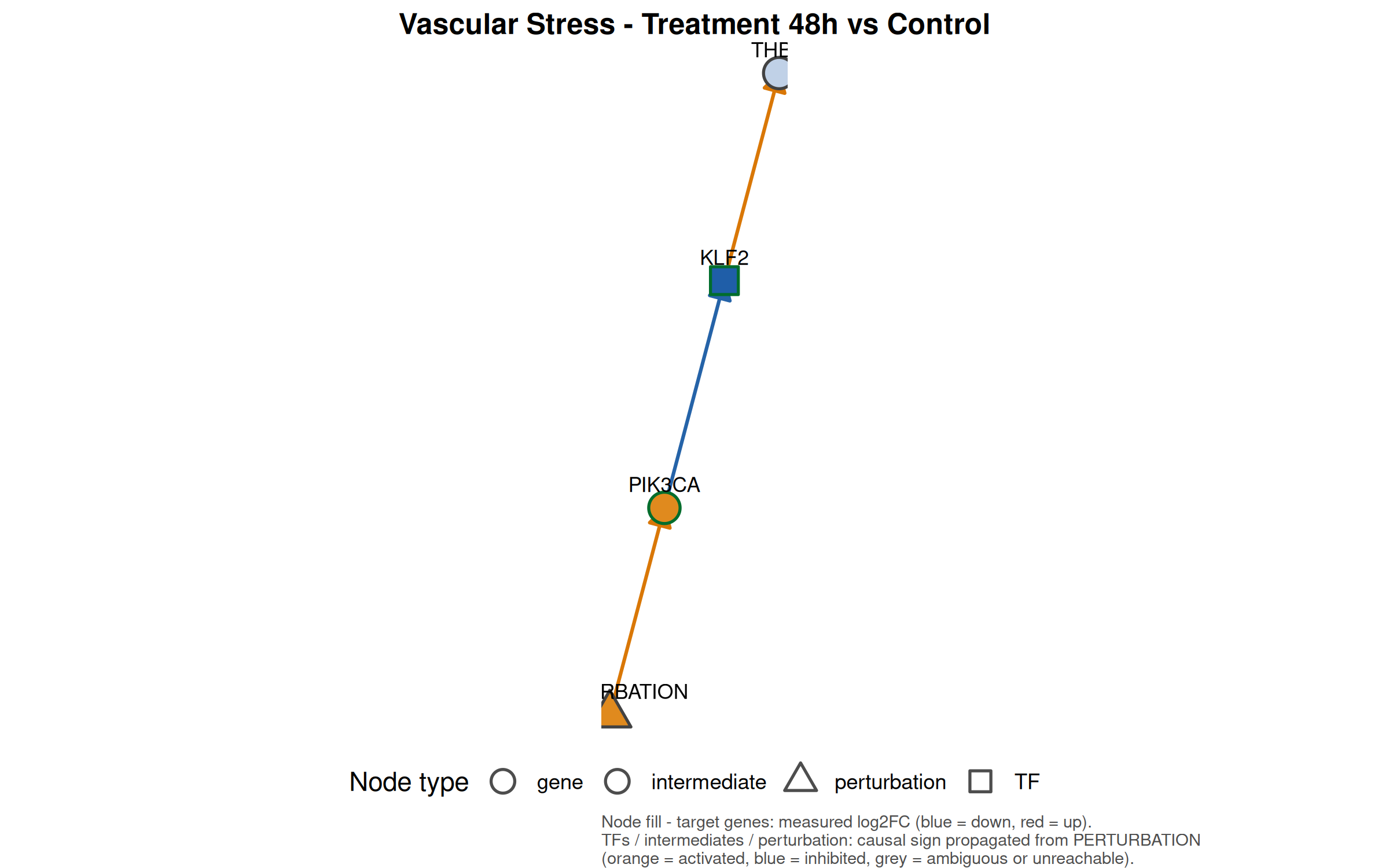
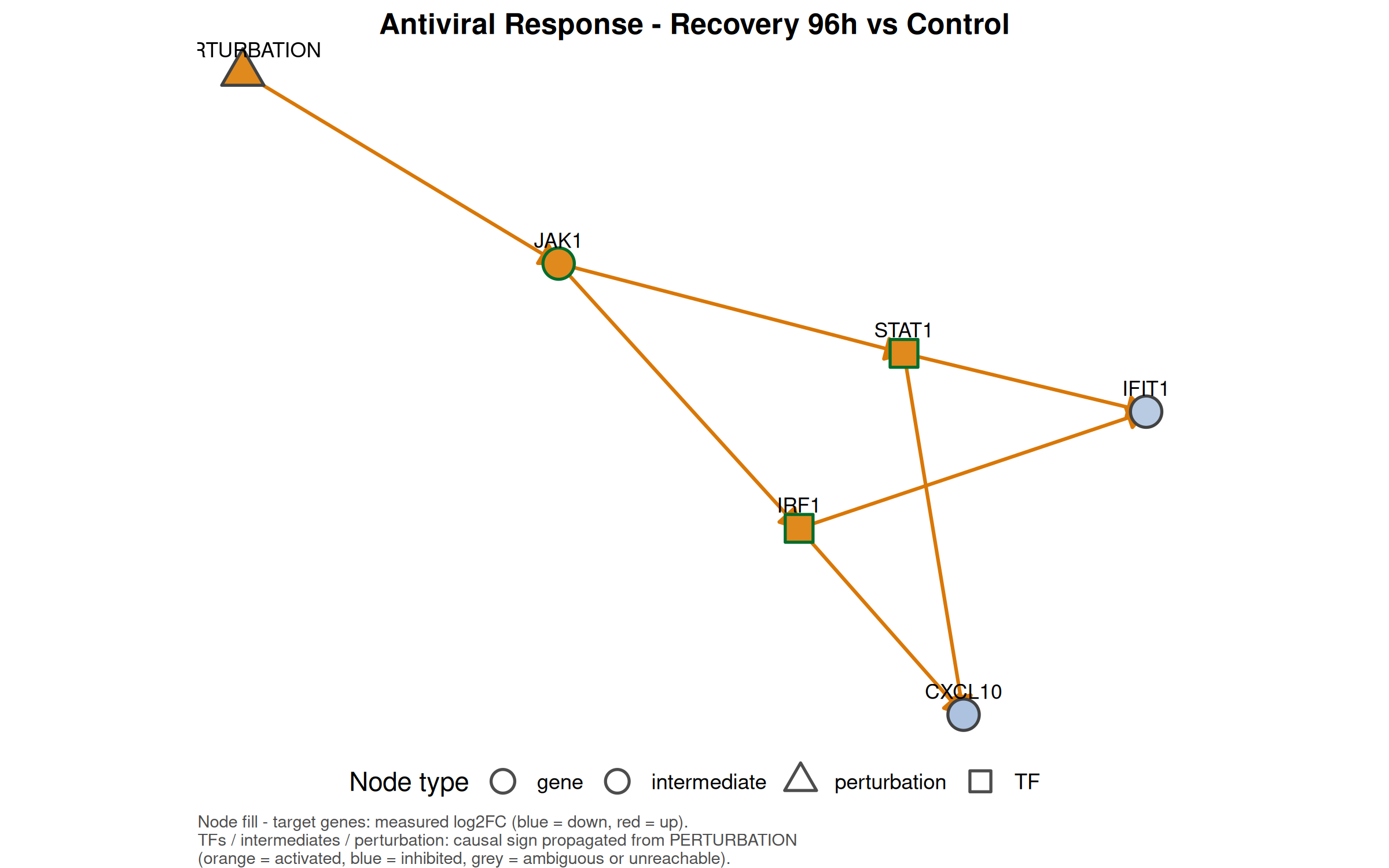
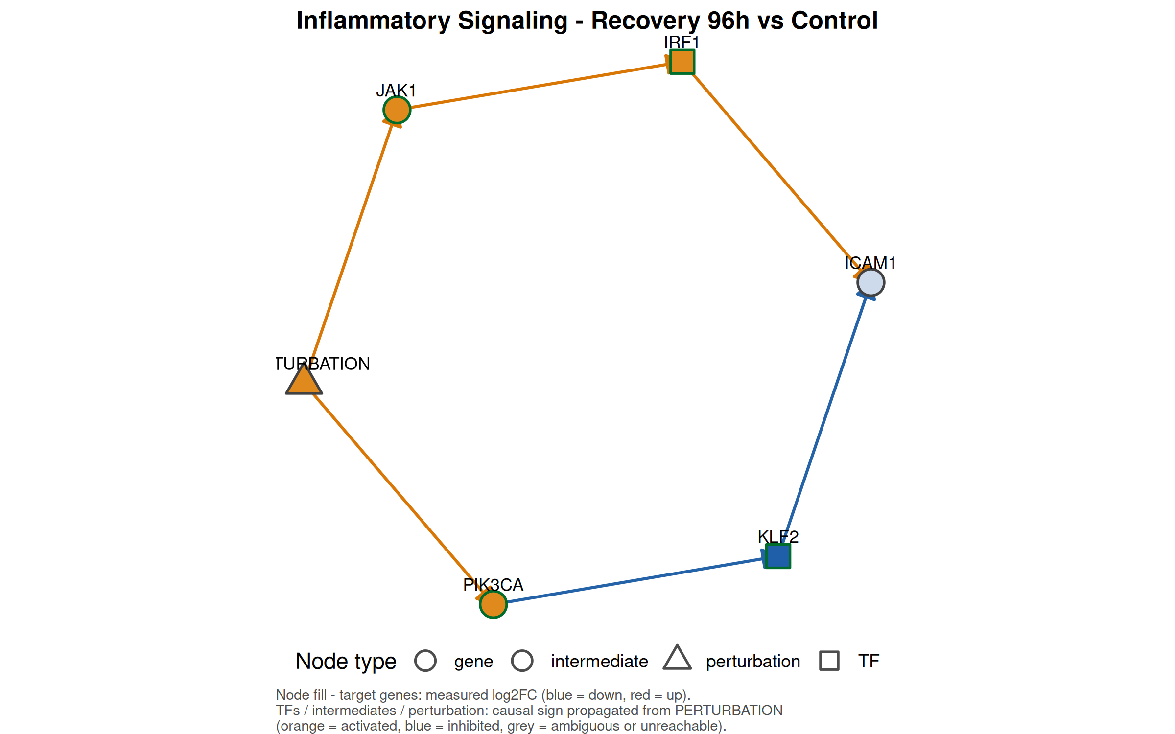
    p <- plot_network(net$edges, net$nodes, paste(str_replace_all(mod, "_", " "), "-", str_replace_all(comp, "_", " ")))
    saved <- save_plot_dual(p, file.path(comp_dir, base), 8, 5)
    print(p)
    module_summary[[paste(comp, mod, sep = "::")]] <- tibble(comparison = comp, module = mod, target_genes_included = paste(sort(unique(net$targets)), collapse = ";"), tfs_included = paste(sort(unique(net$tfs)), collapse = ";"), node_count = nrow(net$nodes), edge_count = nrow(net$edges), png = unname(saved["png"]), svg = unname(saved["svg"]), dot = paste0(sidecar_prefix, ".dot"), sif = paste0(sidecar_prefix, ".sif"))
  }
}

Code
module_summary_tbl <- bind_rows(module_summary)
if (!nrow(module_summary_tbl)) module_summary_tbl <- tibble(comparison = character(), module = character(), target_genes_included = character(), tfs_included = character(), node_count = integer(), edge_count = integer(), png = character(), svg = character(), dot = character(), sif = character())
write_csv(module_summary_tbl, file.path(paths$tables, "module_network_summary.csv"))
module_summary_tbl
# A tibble: 8 × 10
  comparison     module target_genes_included tfs_included node_count edge_count
  <chr>          <chr>  <chr>                 <chr>             <int>      <int>
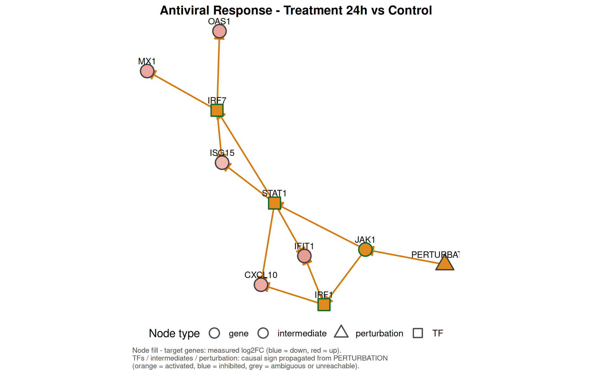
1 Treatment_24h… Antiv… Cxcl10;Ifit1;Irf7;Is… IRF1;IRF7;S…         10         12
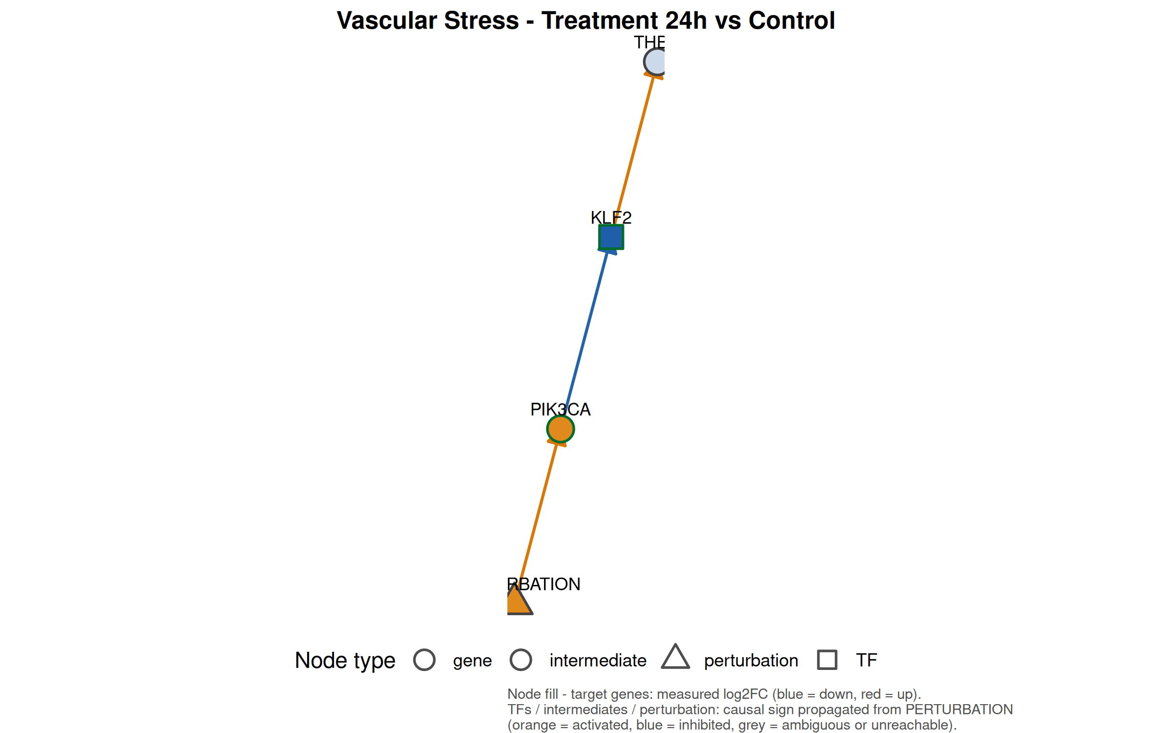
2 Treatment_24h… Vascu… Thbd                  KLF2                  4          3
3 Treatment_48h… Infla… Ccl2;Icam1;Ptgs2;Tnf… KLF2;NFKB1            9         10
4 Treatment_48h… Vascu… Nos2;Thbd;Vegfa       KLF2                  4          3
5 Treatment_48h… Leuko… Itgam;Lyz2;S100a9     SPI1                  0          0
6 Recovery_96h_… Antiv… Cxcl10;Ifit1          IRF1;STAT1            6          7
7 Recovery_96h_… Infla… Icam1                 IRF1;KLF2             6          6
8 Recovery_96h_… Vascu… Angpt2;Thbd           KLF2                  4          3
# ℹ 4 more variables: png <chr>, svg <chr>, dot <chr>, sif <chr>

Module DEG Summary

Code
module_deg_summary <- deg_all %>%
  mutate(gene_upper = harmonize_symbol(Gene)) %>%
  inner_join(modules %>% mutate(gene_upper = harmonize_symbol(gene)), by = "gene_upper") %>%
  filter(significant) %>%
  transmute(module, gene = Gene, Comparison, log2FoldChange, padj, direction = ifelse(log2FoldChange > 0, "up", "down")) %>%
  arrange(module, gene, Comparison)
module_deg_summary %>%
  head(15) %>%
  knitr::kable(
    caption   = "Significant Module DEGs (First 15 Rows)",
    col.names = c("Module", "Gene Symbol", "Comparison", "Log2 Fold Change", "FDR adj. p", "Direction"),
    digits    = 4
  )
Significant Module DEGs (First 15 Rows)
Module Gene Symbol Comparison Log2 Fold Change FDR adj. p Direction
Antiviral_Response Cxcl10 Treatment_24h_vs_Control 2.3740 0.0042 up
Antiviral_Response Cxcl10 Recovery_96h_vs_Control -2.6432 0.0035 down
Antiviral_Response Ifit1 Treatment_24h_vs_Control 2.7982 0.0042 up
Antiviral_Response Ifit1 Recovery_96h_vs_Control -2.2686 0.0043 down
Antiviral_Response Irf7 Treatment_24h_vs_Control 2.2531 0.0042 up
Antiviral_Response Isg15 Treatment_24h_vs_Control 1.9388 0.0037 up
Antiviral_Response Mx1 Treatment_24h_vs_Control 2.4598 0.0042 up
Antiviral_Response Oas1 Treatment_24h_vs_Control 2.6131 0.0011 up
ECM_Remodeling Col4a1 Recovery_96h_vs_Control 1.9717 0.0033 up
ECM_Remodeling Mmp3 Treatment_48h_vs_Control 2.3894 0.0019 up
ECM_Remodeling Mmp3 Recovery_96h_vs_Control 2.2368 0.0026 up
ECM_Remodeling Mmp9 Treatment_48h_vs_Control 1.8362 0.0007 up
ECM_Remodeling Mmp9 Recovery_96h_vs_Control 2.2992 0.0033 up
ECM_Remodeling Spp1 Recovery_96h_vs_Control 1.9081 0.0026 up
Inflammatory_Signaling Ccl2 Treatment_48h_vs_Control 1.8193 0.0015 up