09 · WGCNA Co-Expression Analysis

Weighted gene co-expression network, module–trait correlation, hub genes, and enrichment

DESeqDataSet input. Soft-thresholding power selection, blockwiseModules network construction, module–trait correlation heatmap, eigengene trajectories, hub gene ranking (kME + kWithin + GS), and gprofiler2 enrichment per module. Outputs TIFF/PDF figures and CSV tables.

Overview

Item	Details
Input	dds_wgcna_template.RData — a saved DESeqDataSet already processed with DESeq()
Key packages	WGCNA, DESeq2, gprofiler2, igraph, ggplot2, patchwork
Statistics	Bicor correlation · scale-free topology fit · module–trait Pearson r (FDR) · hub score (kME + z.kWithin + GS.virus)
Output	Dendrogram · module–trait heatmap · eigengene trajectories · correlation barplot · enrichment lollipop · hub gene bubble plot
Download	template.Rmd

Edit the ## ── USER CONFIGURATION block at the top of template.Rmd. At minimum: set DDS_FILE to your saved DESeqDataSet, VIRAL_GENE to the key gene used as a trait (or NULL to skip), and ORGANISM to the gprofiler2 code for your species ("mmusculus" or "hsapiens").

← Gallery Download .Rmd

## ── USER CONFIGURATION ──────────────────────────────────────────────────────
#
# ── Input ────────────────────────────────────────────────────────────────────
DDS_FILE      <- "data/dds_wgcna_template.RData"  # saved DESeqDataSet (post DESeq())
VIRAL_GENE    <- "SIM_VIRUS"     # gene to use as viral-load trait; set NULL to skip
TREATMENT_COL <- "treatment"     # colData column for treatment
VIRUS_LEVEL   <- "virus"         # infected level name
PBS_LEVEL     <- "pbs"           # mock/control level name
DPI_COL       <- "dpi"           # colData column for time point
DPI_MAP       <- c(one = 1, three = 3, five = 5)  # text → numeric dpi; set NULL if already numeric

# ── Enrichment ───────────────────────────────────────────────────────────────
ORGANISM      <- "mmusculus"     # gprofiler2 organism code ("hsapiens" for human)

# ── WGCNA network ───────────────────────────────────────────────────────────
N_THREADS     <- 2               # parallel threads for blockwiseModules
EXPR_FILTER   <- 5               # remove genes with mean VST < this (VST scale ~= log2; typical range 6–15)
VAR_FILTER    <- 0.5             # keep top fraction by MAD (0–1)
SOFT_R2       <- 0.80            # scale-free R² target for power selection
MIN_MOD_SIZE  <- 20              # minimum genes per module
MERGE_HEIGHT  <- 0.25            # module merge dendrogram cut height

# ── Filtering ────────────────────────────────────────────────────────────────
R_CUT         <- 0.6             # |r| threshold for trait-correlated modules
P_CUT         <- 0.05            # FDR p-value threshold

# ── Load and VST-normalize ───────────────────────────────────────────────────
load(DDS_FILE)   # loads object named 'dds'

vst_data    <- varianceStabilizingTransformation(dds, blind = TRUE)
expr_full   <- assay(vst_data)

# Keep viral gene before filtering
if (!is.null(VIRAL_GENE) && VIRAL_GENE %in% rownames(expr_full)) {
  viral_row <- expr_full[VIRAL_GENE, , drop = FALSE]
} else {
  viral_row <- NULL
  if (!is.null(VIRAL_GENE))
    message("VIRAL_GENE '", VIRAL_GENE, "' not found — GS.virus will be skipped.")
  VIRAL_GENE <- NULL
}

# Expression filter
keep_expr  <- rowMeans(expr_full) > EXPR_FILTER
expr_full  <- expr_full[keep_expr, , drop = FALSE]
cat("After expression filter:", nrow(expr_full), "genes\n")

After expression filter: 553 genes

# Variance filter (top VAR_FILTER fraction by MAD)
mad_vals   <- apply(expr_full, 1, mad, na.rm = TRUE)
keep_n     <- floor(length(mad_vals) * VAR_FILTER)
expr_mat   <- expr_full[order(mad_vals, decreasing = TRUE)[seq_len(keep_n)], , drop = FALSE]

# Re-attach viral gene if it was dropped
if (!is.null(viral_row) && !(VIRAL_GENE %in% rownames(expr_mat))) {
  expr_mat <- rbind(expr_mat, viral_row)
}
cat("After variance filter:", nrow(expr_mat), "genes retained\n")

After variance filter: 277 genes retained

Sample Quality Check

datExpr <- t(expr_mat)

# Remove bad samples / genes
gsg <- goodSamplesGenes(datExpr, verbose = 0)
if (!gsg$allOK) {
  datExpr <- datExpr[gsg$goodSamples, gsg$goodGenes]
  message("Removed ", sum(!gsg$goodSamples), " bad samples and ",
          sum(!gsg$goodGenes), " bad genes.")
}

# Sample clustering dendrogram
sampleTree <- hclust(dist(datExpr), method = "average")
par(mar = c(3, 4, 2, 1))
plot(sampleTree,
     main  = "Sample clustering — detect outliers",
     sub   = "", xlab = "", cex = 0.8)

Soft-Thresholding Power

enableWGCNAThreads(N_THREADS)

Allowing parallel execution with up to 2 working processes.

powers <- 1:20
sft <- pickSoftThreshold(
  datExpr,
  powerVector = powers,
  networkType = "signed",
  corFnc      = "bicor",
  corOptions  = list(maxPOutliers = 0.05),
  verbose     = 0
)

   Power SFT.R.sq  slope truncated.R.sq mean.k. median.k. max.k.
1      1  0.18900  3.370          0.749  142.00    142.00  155.0
2      2  0.17600  2.970          0.829   86.30     86.60  104.0
3      3  0.06130  0.906          0.803   58.00     57.80   79.8
4      4  0.00245  0.129          0.670   41.90     41.00   64.5
5      5  0.02150 -0.319          0.437   31.70     30.40   53.8
6      6  0.01750 -0.142          0.410   24.80     23.40   45.8
7      7  0.05990 -0.150          0.539   20.00     18.20   39.4
8      8  0.28200 -0.325          0.580   16.40     14.30   35.3
9      9  0.58500 -0.533          0.718   13.70     11.50   32.2
10    10  0.69200 -0.631          0.791   11.50      9.38   29.5
11    11  0.71500 -0.703          0.730    9.81      7.68   27.1
12    12  0.77200 -0.794          0.784    8.42      6.32   24.9
13    13  0.84500 -0.828          0.864    7.29      5.19   23.0
14    14  0.87500 -0.921          0.874    6.34      4.30   21.3
15    15  0.85300 -0.939          0.842    5.55      3.60   19.7
16    16  0.82100 -0.987          0.786    4.88      3.04   18.2
17    17  0.86600 -0.990          0.841    4.31      2.62   16.9
18    18  0.90500 -1.000          0.896    3.83      2.22   15.7
19    19  0.89800 -1.010          0.884    3.41      1.88   14.6
20    20  0.89000 -1.080          0.869    3.04      1.66   13.6

# Auto-select smallest power reaching SOFT_R2
r_sq   <- -sign(sft$fitIndices$slope) * sft$fitIndices$SFT.R.sq
idx    <- which(r_sq >= SOFT_R2)[1]
softPower <- if (!is.na(idx)) sft$fitIndices$Power[idx] else sft$fitIndices$Power[which.max(r_sq)]
cat("Selected soft-thresholding power:", softPower,
    sprintf("(R² = %.2f, mean connectivity = %.1f)\n",
            r_sq[which(sft$fitIndices$Power == softPower)],
            sft$fitIndices$mean.k.[which(sft$fitIndices$Power == softPower)]))

Selected soft-thresholding power: 13 (R² = 0.84, mean connectivity = 7.3)

par(mfrow = c(1, 2), mar = c(4, 4, 2, 1))
plot(sft$fitIndices[, 1], r_sq,
     xlab = "Soft threshold (power)", ylab = "Scale-free R²",
     main = "Scale independence", type = "b", pch = 19)
abline(h = SOFT_R2, lty = 2)
plot(sft$fitIndices[, 1], sft$fitIndices[, 5],
     xlab = "Soft threshold (power)", ylab = "Mean connectivity",
     main = "Mean connectivity", type = "b", pch = 19)

par(mfrow = c(1, 1), mar = c(5.1, 4.1, 4.1, 2.1))

Network Construction

set.seed(1234)
dir.create("WGCNA_data", showWarnings = FALSE)

net <- blockwiseModules(
  datExpr,
  power            = softPower,
  networkType      = "signed",
  TOMType          = "signed",
  corType          = "bicor",
  minModuleSize    = MIN_MOD_SIZE,
  reassignThreshold = 0,
  mergeCutHeight   = MERGE_HEIGHT,
  maxBlockSize     = 25000,
  numericLabels    = FALSE,
  pamRespectsDendro = TRUE,
  saveTOMs         = FALSE,
  verbose          = 0,
  nThreads         = N_THREADS
)

moduleColors <- labels2colors(net$colors)
cat("Modules detected:", length(unique(moduleColors[moduleColors != "grey"])), "\n")
cat("Grey (unassigned) genes:", sum(moduleColors == "grey"), "\n")

Module Dendrogram

dir.create("Plots", showWarnings = FALSE)

tiff("Plots/WGCNA_Dendrogram.tiff",
     width = 5, height = 3, units = "in",
     res = 300, compression = "lzw",
     family = "Arial", pointsize = 10)
par(mar = c(1, 4.1, 2.5, 1))
plotDendroAndColors(
  net$dendrograms[[1]],
  moduleColors[net$blockGenes[[1]]],
  groupLabels  = "Module",
  dendroLabels = FALSE,
  main         = "Cluster Dendrogram",
  addGuide     = TRUE,
  hang         = 0.03
)
dev.off()

png 
  2 

plotDendroAndColors(
  net$dendrograms[[1]],
  moduleColors[net$blockGenes[[1]]],
  groupLabels  = "Module",
  dendroLabels = FALSE,
  main         = "Cluster Dendrogram",
  addGuide     = TRUE,
  hang         = 0.03
)

# Save module assignments
gene_names       <- colnames(datExpr)
module_assignments <- data.frame(
  Gene   = gene_names,
  Module = moduleColors,
  stringsAsFactors = FALSE
)
dir.create("Gene_sets", showWarnings = FALSE)
write.csv(module_assignments, "Gene_sets/module_assignments.csv", row.names = FALSE)
cat("Module assignments saved (", nrow(module_assignments), "genes )\n")

Module assignments saved ( 277 genes )

Module–Trait Correlation

MEs         <- orderMEs(net$MEs)
# Subset colData to the samples that survived gsg filtering
sampleInfo  <- as.data.frame(colData(dds))[rownames(datExpr), , drop = FALSE]

# Build numeric trait data
traitData <- data.frame(
  dpi       = if (!is.null(DPI_MAP)) DPI_MAP[sampleInfo[[DPI_COL]]] else as.numeric(sampleInfo[[DPI_COL]]),
  infection = as.numeric(sampleInfo[[TREATMENT_COL]] == VIRUS_LEVEL),
  row.names = rownames(sampleInfo)
)

if (!is.null(VIRAL_GENE) && VIRAL_GENE %in% rownames(assay(vst_data))) {
  traitData$virus <- as.numeric(assay(vst_data)[VIRAL_GENE, rownames(sampleInfo)])
}

moduleTraitCor <- cor(MEs, traitData, use = "pairwise.complete.obs")
moduleTraitPvalue <- corPvalueStudent(moduleTraitCor, nSamples = nrow(MEs))
moduleTraitPvalue <- apply(moduleTraitPvalue, 2, p.adjust, method = "fdr")

# Reorder rows by viral load correlation (or infection if no viral gene)
ord_col  <- if ("virus" %in% colnames(moduleTraitCor)) "virus" else "infection"
ord      <- order(moduleTraitCor[, ord_col], decreasing = TRUE)

trait_labels <- c(dpi = "Days post-infection",
                  infection = "Infection (virus vs PBS)",
                  virus = "Viral RNA (RNA-seq)")
x_labels <- trait_labels[colnames(moduleTraitCor)]

stars <- ifelse(moduleTraitPvalue[ord, ] < 0.001, "***",
         ifelse(moduleTraitPvalue[ord, ] < 0.01,  "**",
         ifelse(moduleTraitPvalue[ord, ] < 0.05,  "*", "ns")))
dim(stars) <- dim(moduleTraitPvalue[ord, ])

y_labs <- gsub("^ME", "", rownames(moduleTraitCor)[ord])

plot_file <- "Plots/WGCNA_ModuleTraitHeatmap.pdf"
cairo_pdf(plot_file, width = 2.5, height = 5.5, family = "Arial", pointsize = 10)
par(mar = c(5, 6, 2, 1), cex.main = 0.9)
labeledHeatmap(
  Matrix          = moduleTraitCor[ord, ],
  xLabels         = x_labels,
  yLabels         = y_labs,
  colorLabels     = TRUE,
  colors          = blueWhiteRed(50),
  textMatrix      = stars,
  setStdMargins   = FALSE,
  cex.text        = 0.9,
  cex.lab         = 0.7,
  main            = "Module–Trait Correlation",
  zlim            = c(-1, 1)
)
dev.off()

png 
  2 

par(mar = c(5, 6, 2, 1), cex.main = 0.9)
labeledHeatmap(
  Matrix          = moduleTraitCor[ord, ],
  xLabels         = x_labels,
  yLabels         = y_labs,
  colorLabels     = TRUE,
  colors          = blueWhiteRed(50),
  textMatrix      = stars,
  setStdMargins   = FALSE,
  cex.text        = 0.9,
  cex.lab         = 0.7,
  main            = "Module–Trait Correlation",
  zlim            = c(-1, 1)
)

par(mar = c(5.1, 4.1, 4.1, 2.1))

Trait-Correlated Modules

module_df <- data.frame(
  Module      = rownames(moduleTraitCor),
  dpiCor      = moduleTraitCor[, "dpi"],
  infectionCor = moduleTraitCor[, "infection"],
  dpiP        = moduleTraitPvalue[, "dpi"],
  infectionP  = moduleTraitPvalue[, "infection"],
  stringsAsFactors = FALSE
)

if ("virus" %in% colnames(moduleTraitCor)) {
  module_df$virusCor <- moduleTraitCor[, "virus"]
  module_df$virusP   <- moduleTraitPvalue[, "virus"]
} else {
  module_df$virusCor <- module_df$infectionCor
  module_df$virusP   <- module_df$infectionP
}

# Gene counts per module
moduleGeneCounts      <- table(moduleColors)
mod_names_clean       <- gsub("^ME", "", module_df$Module)
module_df$geneCount   <- as.numeric(moduleGeneCounts[mod_names_clean])
module_df$geneCount[is.na(module_df$geneCount)] <- 0

module_df <- module_df %>%
  dplyr::filter(
    !grepl("grey", Module, ignore.case = TRUE),
    geneCount > 0,
    (abs(virusCor) >= R_CUT & virusP < P_CUT) |
    (abs(infectionCor) >= R_CUT & infectionP < P_CUT)
  ) %>%
  dplyr::arrange(desc(abs(virusCor))) %>%
  dplyr::mutate(Module = gsub("^ME", "", Module))

cat("Trait-correlated modules (|r| ≥", R_CUT, "& FDR <", P_CUT, "):",
    nrow(module_df), "\n")

Trait-correlated modules (|r| ≥ 0.6 & FDR < 0.05 ): 2 

print(module_df[, c("Module", "geneCount", "virusCor", "virusP",
                    "infectionCor", "infectionP")], row.names = FALSE)

    Module geneCount   virusCor       virusP infectionCor   infectionP
 turquoise        64  0.9739487 4.915391e-11    0.9695431 1.691940e-10
      blue        52 -0.7196400 1.900346e-03   -0.7044787 2.745598e-03

Module–Virus Correlation Barplot

plot_df_bar <- module_df %>%
  dplyr::mutate(Module = reorder(Module, virusCor))

sig_label <- dplyr::case_when(
  plot_df_bar$virusP < 0.01 ~ paste0(plot_df_bar$geneCount, "**"),
  plot_df_bar$virusP < 0.05 ~ paste0(plot_df_bar$geneCount, "*"),
  TRUE ~ as.character(plot_df_bar$geneCount)
)

p_bar <- ggplot(plot_df_bar, aes(x = Module, y = virusCor, fill = virusCor)) +
  geom_col(width = 0.7) +
  coord_flip() +
  scale_fill_gradient2(
    low = "blue", mid = "white", high = "red",
    midpoint = 0, limits = c(-1, 1), name = "Correlation"
  ) +
  geom_text(aes(
    label = sig_label,
    hjust = ifelse(virusCor > 0, -0.2, 1.2)
  ), size = 2.5) +
  geom_hline(yintercept = 0, color = "grey30") +
  scale_y_continuous(expand = expansion(mult = c(0.2, 0.2))) +
  labs(x = "Module", y = "Correlation with viral expression",
       title = "Module–viral load correlation") +
  theme_classic(base_size = 10, base_family = "Arial") +
  theme(
    plot.title  = element_text(size = 10, face = "bold", hjust = 0.5),
    axis.title  = element_text(size = 9),
    panel.border = element_rect(color = "black", fill = NA, linewidth = 0.5),
    plot.margin = margin(5, 5, 5, 5)
  )

ggsave("Plots/WGCNA_ModuleCor_Barplot.tiff",
       plot = p_bar, width = 4.5, height = 5, units = "in",
       dpi = 300, compression = "lzw")
print(p_bar)

Eigengene Trajectories

modules_keep <- paste0("ME", module_df$Module)

ME_df        <- as.data.frame(net$MEs)
ME_df$sample <- rownames(ME_df)
# Subset colData to the same samples that are in ME_df
meta         <- as.data.frame(colData(dds))[rownames(ME_df), , drop = FALSE]

meta$dpi_n <- if (!is.null(DPI_MAP)) DPI_MAP[meta[[DPI_COL]]] else as.numeric(meta[[DPI_COL]])
plot_df_eig <- cbind(ME_df, meta)

long_df <- plot_df_eig %>%
  tidyr::pivot_longer(cols = starts_with("ME"),
                      names_to = "Module", values_to = "Eigengene") %>%
  dplyr::filter(Module %in% modules_keep) %>%
  dplyr::mutate(
    Module = gsub("^ME", "", Module),
    Module = paste0(toupper(substr(Module, 1, 1)), substr(Module, 2, nchar(Module)))
  ) %>%
  dplyr::group_by(Module, dpi_n, .data[[TREATMENT_COL]]) %>%
  dplyr::summarise(
    meanEig = mean(Eigengene, na.rm = TRUE),
    seEig   = sd(Eigengene, na.rm = TRUE) / sqrt(dplyr::n()),
    .groups = "drop"
  )

# Center virus eigengene against PBS baseline
baseline <- long_df %>%
  dplyr::filter(.data[[TREATMENT_COL]] == PBS_LEVEL) %>%
  dplyr::select(Module, dpi_n, PBS_mean = meanEig)

long_df <- long_df %>%
  dplyr::left_join(baseline, by = c("Module", "dpi_n")) %>%
  dplyr::mutate(meanEig_centered = meanEig - PBS_mean)

p_traj <- ggplot(
    long_df %>% dplyr::filter(.data[[TREATMENT_COL]] == VIRUS_LEVEL),
    aes(x = dpi_n, y = meanEig_centered, group = 1)
  ) +
  geom_hline(yintercept = 0, color = "black", linetype = "dashed", linewidth = 0.5) +
  geom_line(color = "black", linewidth = 0.8) +
  geom_point(color = "black", size = 2) +
  geom_errorbar(aes(ymin = meanEig_centered - seEig,
                    ymax = meanEig_centered + seEig),
                width = 0.2, linewidth = 0.4, color = "black") +
  facet_wrap(~Module, scales = "free_y") +
  scale_x_continuous(breaks = unique(long_df$dpi_n)) +
  labs(x = "Days post-infection", y = "Eigengene (\u0394 vs control)") +
  theme_classic(base_size = 10, base_family = "Arial") +
  theme(
    strip.background = element_blank(),
    strip.text       = element_text(size = 9, face = "bold"),
    axis.title       = element_text(size = 10),
    panel.border     = element_blank()
  )

ggsave("Plots/WGCNA_Eigengene_Trajectories.pdf",
       plot = p_traj, width = 7, height = 5, units = "in", device = cairo_pdf)
print(p_traj)

Hub Gene Analysis

zNA <- function(x) { y <- as.numeric(scale(x)); y[!is.finite(y)] <- 0; y }

keep_mods  <- module_df$Module
keep_genes <- moduleColors %in% keep_mods & moduleColors != "grey"

datExpr_h      <- as.matrix(datExpr[, keep_genes, drop = FALSE])
moduleColors_h <- moduleColors[keep_genes]
geneNames_h    <- colnames(datExpr_h)

MEs_matrix <- as.matrix(orderMEs(net$MEs))
kME_all    <- signedKME(datExpr_h, MEs_matrix,
                         corFnc = "bicor",
                         corOptions = "use = 'p', maxPOutliers = 0.05")
colnames(kME_all) <- sub("^(kME|ME)", "", colnames(kME_all))

mod_idx     <- match(moduleColors_h, colnames(kME_all))
kME_inMod   <- kME_all[cbind(seq_along(geneNames_h), mod_idx)]

adj <- adjacency(datExpr_h, power = softPower, type = "signed",
                 corFnc = "bicor",
                 corOptions = list(maxPOutliers = 0.05, use = "p"))
diag(adj) <- 0
IMC <- intramodularConnectivity(adj, colors = moduleColors_h)
IMC$z.kWithin <- zNA(IMC$kWithin)

hub_tbl <- data.frame(
  Gene      = geneNames_h,
  Module    = moduleColors_h,
  kME       = kME_inMod,
  kWithin   = IMC$kWithin,
  z.kWithin = IMC$z.kWithin,
  stringsAsFactors = FALSE
)

if (!is.null(VIRAL_GENE) && VIRAL_GENE %in% colnames(datExpr_h)) {
  virus_vec      <- as.numeric(datExpr_h[, VIRAL_GENE])
  GS_virus       <- bicor(datExpr_h, virus_vec, maxPOutliers = 0.05,
                          use = "pairwise.complete.obs")
  hub_tbl$GS.virus <- as.numeric(GS_virus)
} else {
  hub_tbl$GS.virus <- 0
}

hub_tbl <- hub_tbl %>%
  dplyr::group_by(Module) %>%
  dplyr::mutate(hubness = zNA(abs(kME)) + zNA(z.kWithin) + zNA(abs(GS.virus))) %>%
  dplyr::ungroup()

hub_summary <- hub_tbl %>%
  dplyr::group_by(Module) %>%
  dplyr::summarise(
    topGene        = Gene[which.max(hubness)],
    meanHubness    = mean(hubness, na.rm = TRUE),
    maxHubness     = max(hubness, na.rm = TRUE),
    meanAbsGSvirus = mean(abs(GS.virus), na.rm = TRUE),
    .groups = "drop"
  )

module_df <- module_df %>% dplyr::left_join(hub_summary, by = "Module")

dir.create("WGCNA_data/hubs", showWarnings = FALSE, recursive = TRUE)
write.csv(hub_tbl,     "WGCNA_data/hubs/hub_genes_filtered_modules.csv",  row.names = FALSE)
write.csv(hub_summary, "WGCNA_data/hubs/hub_summary_by_module.csv",        row.names = FALSE)

cat("Hub analysis complete. Top hub genes per module:\n")

Hub analysis complete. Top hub genes per module:

print(module_df[, c("Module", "geneCount", "topGene", "maxHubness", "virusCor")],
      row.names = FALSE)

    Module geneCount    topGene maxHubness   virusCor
 turquoise        64   Blue_G17   2.931312  0.9739487
      blue        52 Yellow_G28   2.685363 -0.7196400

Enrichment Analysis (gprofiler2)

filtered_mods <- unique(module_df$Module)
cat("Running enrichment for", length(filtered_mods), "modules\n")

Running enrichment for 2 modules

out_dir <- "WGCNA_data/enrichment"
dir.create(out_dir, recursive = TRUE, showWarnings = FALSE)

results_list <- lapply(filtered_mods, function(mod) {
  genes_in_module <- module_assignments$Gene[module_assignments$Module == mod]
  if (length(genes_in_module) < 10) return(NULL)

  gostres <- tryCatch(
    gost(
      query            = genes_in_module,
      significant      = TRUE,
      correction_method = "fdr",
      organism         = ORGANISM,
      sources          = c("GO:BP", "GO:MF", "GO:CC", "KEGG", "REAC", "WP",
                           "MIRNA", "TF", "CORUM")
    ),
    error = function(e) { message("Enrichment error (module ", mod, "): ", e$message); NULL }
  )

  if (is.null(gostres) || is.null(gostres$result)) return(NULL)

  gostres$result %>%
    dplyr::mutate(gene_count = intersection_size, module = mod) %>%
    dplyr::mutate(dplyr::across(where(is.list),
      ~ sapply(., function(x) paste(unlist(x), collapse = "; ")))) %>%
    dplyr::filter(term_size >= 10 & term_size <= 2000) %>%
    dplyr::arrange(p_value)
})

all_enrich <- dplyr::bind_rows(results_list)
if (nrow(all_enrich) > 0) {
  write.csv(all_enrich,
            file.path(out_dir, "gprofiler_all_terms.csv"), row.names = FALSE)
  cat("Enrichment results written:", nrow(all_enrich), "terms across",
      length(unique(all_enrich$module)), "modules\n")

  top_per_source <- all_enrich %>%
    dplyr::group_by(module, source) %>%
    dplyr::slice_min(p_value, n = 1, with_ties = FALSE) %>%
    dplyr::ungroup() %>%
    dplyr::select(module, source, term_name, p_value, gene_count, term_size)

  print(top_per_source, n = Inf)
} else {
  cat("No significant enrichment terms found.\n")
}

No significant enrichment terms found.

Enrichment Lollipop Plot

if (nrow(all_enrich) > 0) {
  order_df <- all_enrich %>%
    dplyr::mutate(
      gene_ratio = gene_count / term_size,
      logFDR     = -log10(p_value)
    ) %>%
    dplyr::arrange(module, p_value) %>%
    dplyr::group_by(module) %>%
    dplyr::slice_head(n = 3) %>%
    dplyr::ungroup() %>%
    dplyr::mutate(y_id = dplyr::row_number())

  seps_df <- order_df %>% dplyr::count(module) %>%
    dplyr::mutate(cum = cumsum(n), yint = cum + 0.5)
  labs_df <- order_df %>% dplyr::count(module) %>%
    dplyr::mutate(y_mid = cumsum(n) - n / 2)
  x_right <- max(order_df$gene_ratio, na.rm = TRUE) * 1.05

  p_lollipop <- ggplot(order_df, aes(x = gene_ratio, y = y_id)) +
    geom_segment(aes(x = 0, xend = gene_ratio, yend = y_id),
                 linewidth = 0.4, color = "grey70") +
    geom_point(aes(size = gene_count, color = logFDR)) +
    geom_hline(data = seps_df, aes(yintercept = yint),
               inherit.aes = FALSE, color = "grey85", linewidth = 0.3) +
    geom_text(data = labs_df, aes(x = x_right, y = y_mid, label = module),
              inherit.aes = FALSE, hjust = 0, size = 3) +
    scale_y_continuous(breaks = order_df$y_id, labels = order_df$term_name) +
    scale_size_area(max_size = 6, name = "Hit genes") +
    scale_color_viridis_c(name = expression("-log"[10] * "(FDR)")) +
    scale_x_continuous(labels = scales::percent_format(accuracy = 1),
                       expand = expansion(mult = c(0, 0.05))) +
    coord_cartesian(clip = "off") +
    expand_limits(x = x_right) +
    labs(x = "Gene ratio (%)", y = NULL, title = "Top enriched terms per module") +
    theme_bw(base_size = 10, base_family = "Arial") +
    theme(
      panel.grid.major = element_blank(),
      panel.grid.minor = element_blank(),
      axis.text.y  = element_text(size = 7),
      plot.margin  = margin(5, 40, 5, 5)
    )

  ggsave("Plots/WGCNA_Enrichment_Lollipop.pdf",
         plot = p_lollipop, width = 7, height = 6, device = cairo_pdf)
  print(p_lollipop)
} else {
  message("Skipping lollipop plot — no enrichment results.")
}

Hub Gene Bubble Plot

# DE results per DPI contrast (virus vs PBS).
# Names must match keys in DPI_MAP; values assume group = paste0(treatment, dpi).
# Update these if your group encoding differs.
dpi_contrasts <- list(
  one   = c("group", paste0(VIRUS_LEVEL, "one"),   paste0(PBS_LEVEL, "one")),
  three = c("group", paste0(VIRUS_LEVEL, "three"), paste0(PBS_LEVEL, "three")),
  five  = c("group", paste0(VIRUS_LEVEL, "five"),  paste0(PBS_LEVEL, "five"))
)

tidy_res <- function(res, dpi_val) {
  as.data.frame(res) %>%
    tibble::rownames_to_column("Gene") %>%
    dplyr::transmute(Gene, dpi = dpi_val, log2FoldChange, padj)
}

de_long <- dplyr::bind_rows(
  lapply(names(dpi_contrasts), function(d) {
    tryCatch(
      tidy_res(results(dds, contrast = dpi_contrasts[[d]]), DPI_MAP[d]),
      error = function(e) NULL
    )
  })
)

DEG_genes <- de_long %>%
  dplyr::filter(!is.na(padj), padj < 0.05, abs(log2FoldChange) >= 0.5) %>%
  dplyr::distinct(Gene) %>%
  dplyr::pull(Gene)
cat("Genes passing DEG filter:", length(DEG_genes), "\n")

Genes passing DEG filter: 239 

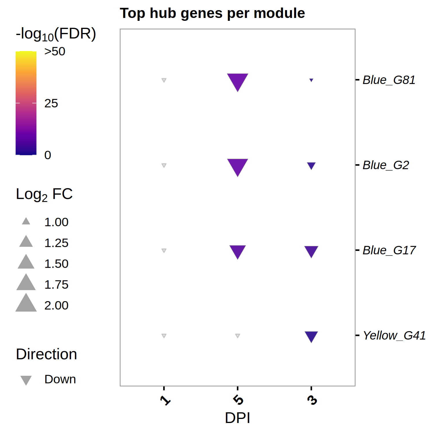
# Top 3 hub genes per module (from DEG set)
top3 <- hub_tbl %>%
  dplyr::filter(Gene %in% DEG_genes) %>%
  dplyr::arrange(Module, dplyr::desc(hubness)) %>%
  dplyr::group_by(Module) %>%
  dplyr::slice_head(n = 3) %>%
  dplyr::ungroup() %>%
  dplyr::select(Gene, Module)

if (nrow(top3) == 0) {
  message("No hub genes overlap with DEGs — all genes will be shown.")
  top3 <- hub_tbl %>%
    dplyr::arrange(Module, dplyr::desc(hubness)) %>%
    dplyr::group_by(Module) %>%
    dplyr::slice_head(n = 3) %>%
    dplyr::ungroup() %>%
    dplyr::select(Gene, Module)
}

ordered_genes <- top3 %>% dplyr::arrange(Module, Gene) %>% dplyr::pull(Gene) %>% unique()

plot_bubble <- de_long %>%
  dplyr::inner_join(top3, by = "Gene") %>%
  dplyr::mutate(
    Comparison  = factor(as.character(dpi), levels = as.character(sort(unique(dpi)))),
    Gene        = factor(Gene, levels = ordered_genes),
    color_group = ifelse(!is.na(padj) & padj < 0.05, "significant", "nonsignificant"),
    log_padj    = ifelse(!is.na(padj) & padj > 0, -log10(padj), 0),
    direction   = ifelse(log2FoldChange > 0, "Up", "Down")
  )

cap_val <- 50

p_bubble <- ggplot() +
  geom_point(
    data  = dplyr::filter(plot_bubble, color_group == "nonsignificant"),
    aes(x = Comparison, y = Gene),
    shape = 25, size = 0.8, color = "grey60", fill = "grey80", alpha = 0.5
  ) +
  geom_point(
    data  = dplyr::filter(plot_bubble, color_group == "significant"),
    aes(x = Comparison, y = Gene,
        size = abs(log2FoldChange),
        fill = pmin(log_padj, cap_val),
        shape = direction),
    color = "grey60", stroke = 0.2, alpha = 0.9
  ) +
  scale_shape_manual(values = c(Up = 24, Down = 25), name = "Direction",
    guide = guide_legend(override.aes = list(fill = "grey60", size = 3))) +
  scale_size_continuous(name = expression("Log"[2] * " FC"),
    guide = guide_legend(override.aes = list(shape = 24, fill = "grey60"))) +
  scale_fill_viridis_c(
    option = "plasma", name = expression("-log"[10] * "(FDR)"),
    limits = c(0, cap_val), breaks = c(0, 25, cap_val),
    labels = c("0", "25", paste0(">", cap_val))
  ) +
  scale_y_discrete(position = "right", drop = FALSE) +
  labs(title = "Top hub genes per module", x = "DPI", y = NULL) +
  theme_classic(base_size = 13, base_family = "Arial") +
  theme(
    axis.text.x  = element_text(size = 12, angle = 45, hjust = 1, face = "bold"),
    axis.text.y  = element_text(size = 10, face = "italic"),
    legend.position = "left",
    panel.border = element_rect(color = "grey60", fill = NA, linewidth = 0.6),
    axis.line    = element_blank(),
    plot.title   = element_text(size = 12, face = "bold")
  )

ggsave("Plots/WGCNA_HubGene_Bubble.tiff",
       p_bubble, width = 6, height = 5, dpi = 300, compression = "lzw")
ggsave("Plots/WGCNA_HubGene_Bubble.pdf",
       p_bubble, width = 6, height = 5, device = cairo_pdf)
print(p_bubble)