01 · Plaque Assay + Violin Plots

Viral titer quantification with replicate QC and significance testing

infection
virology
ANOVA
plaque-assay

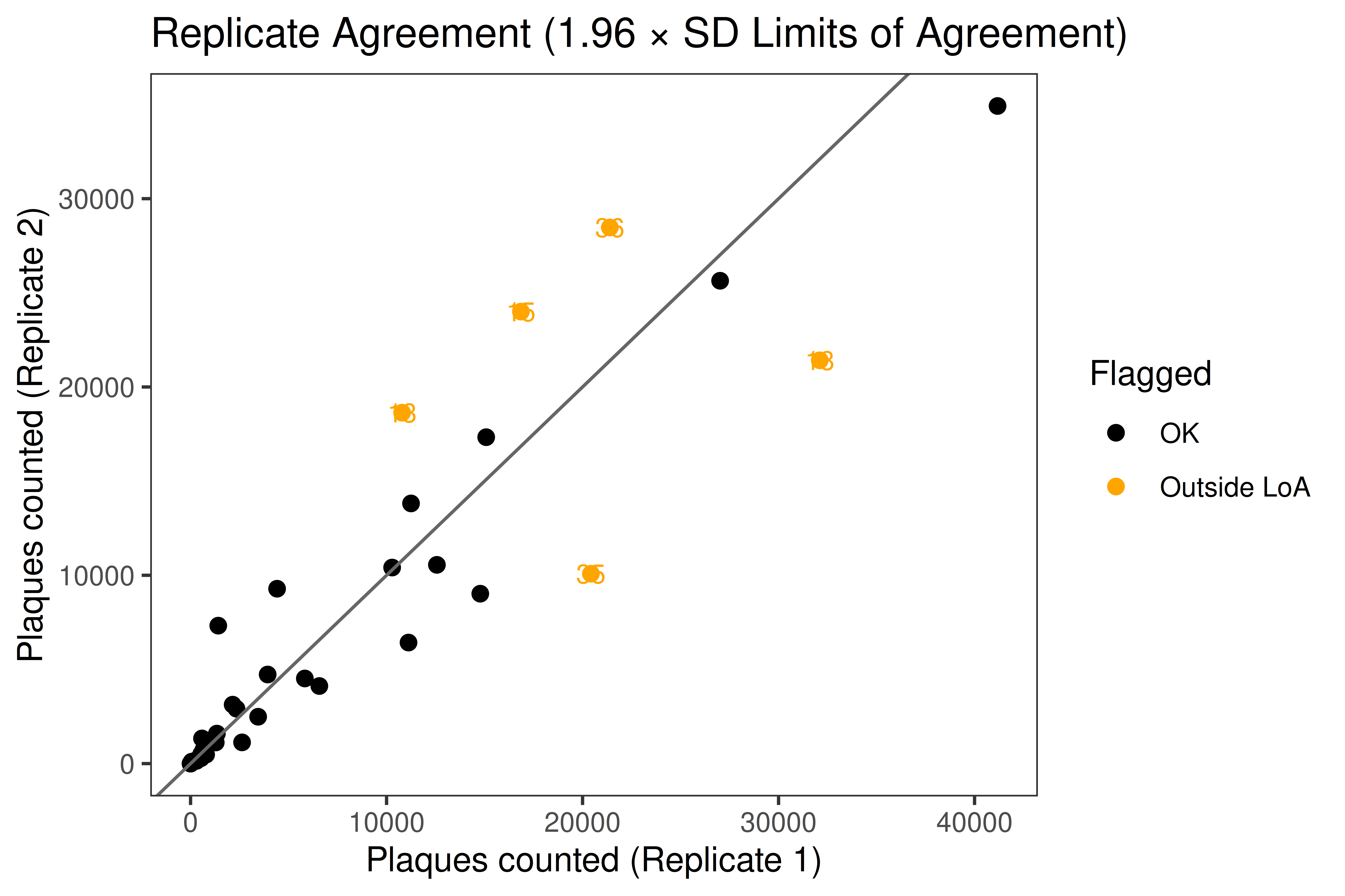
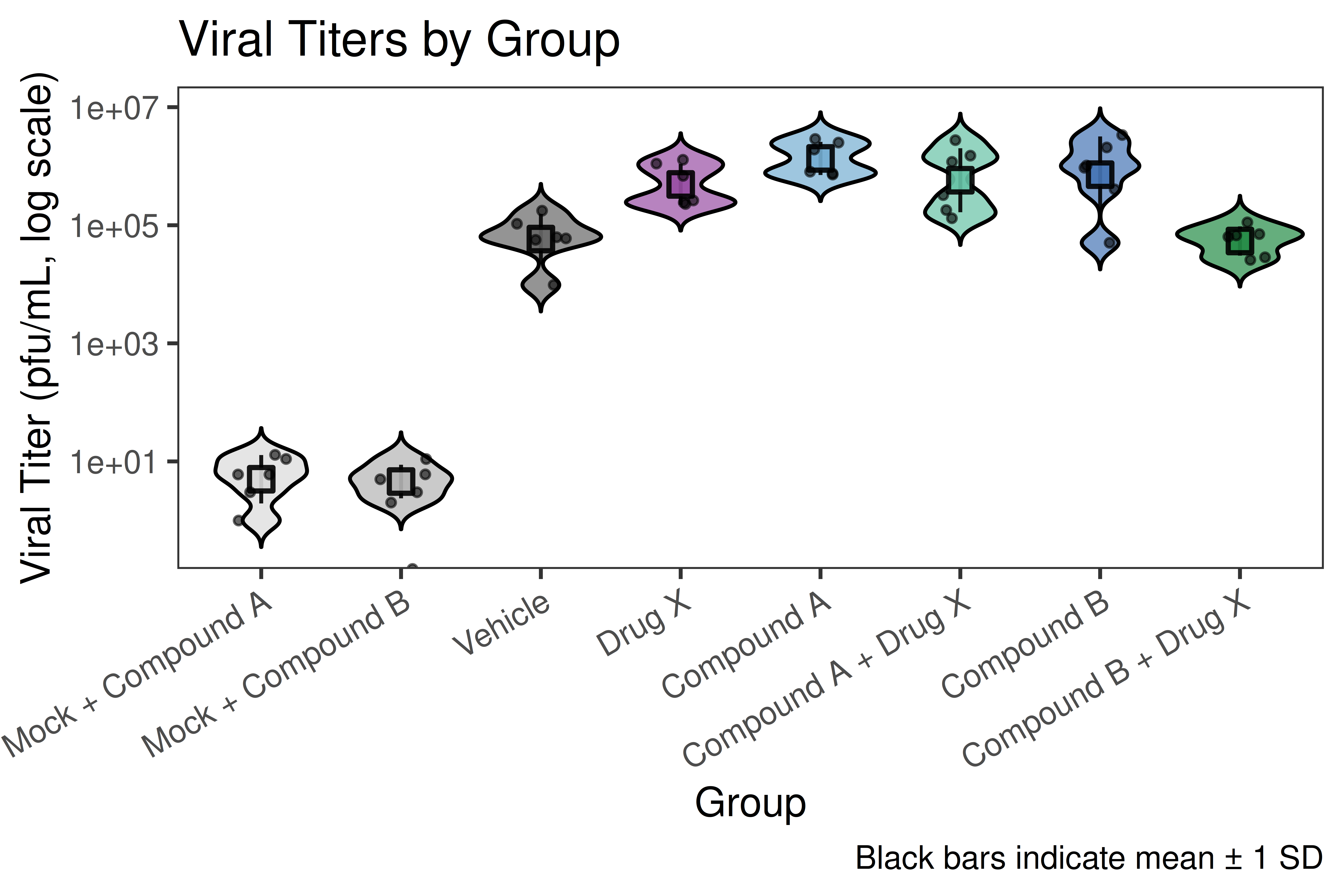
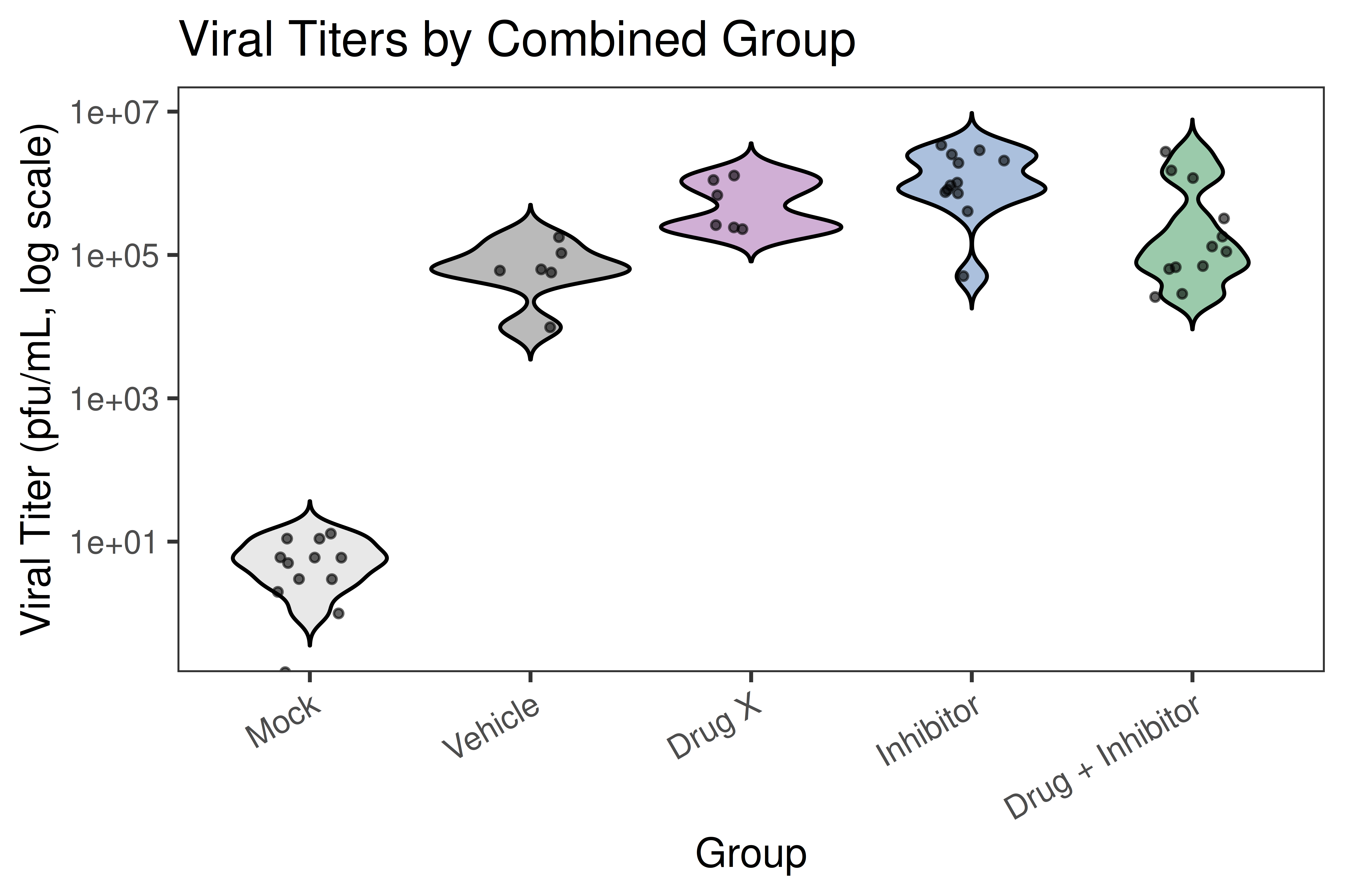
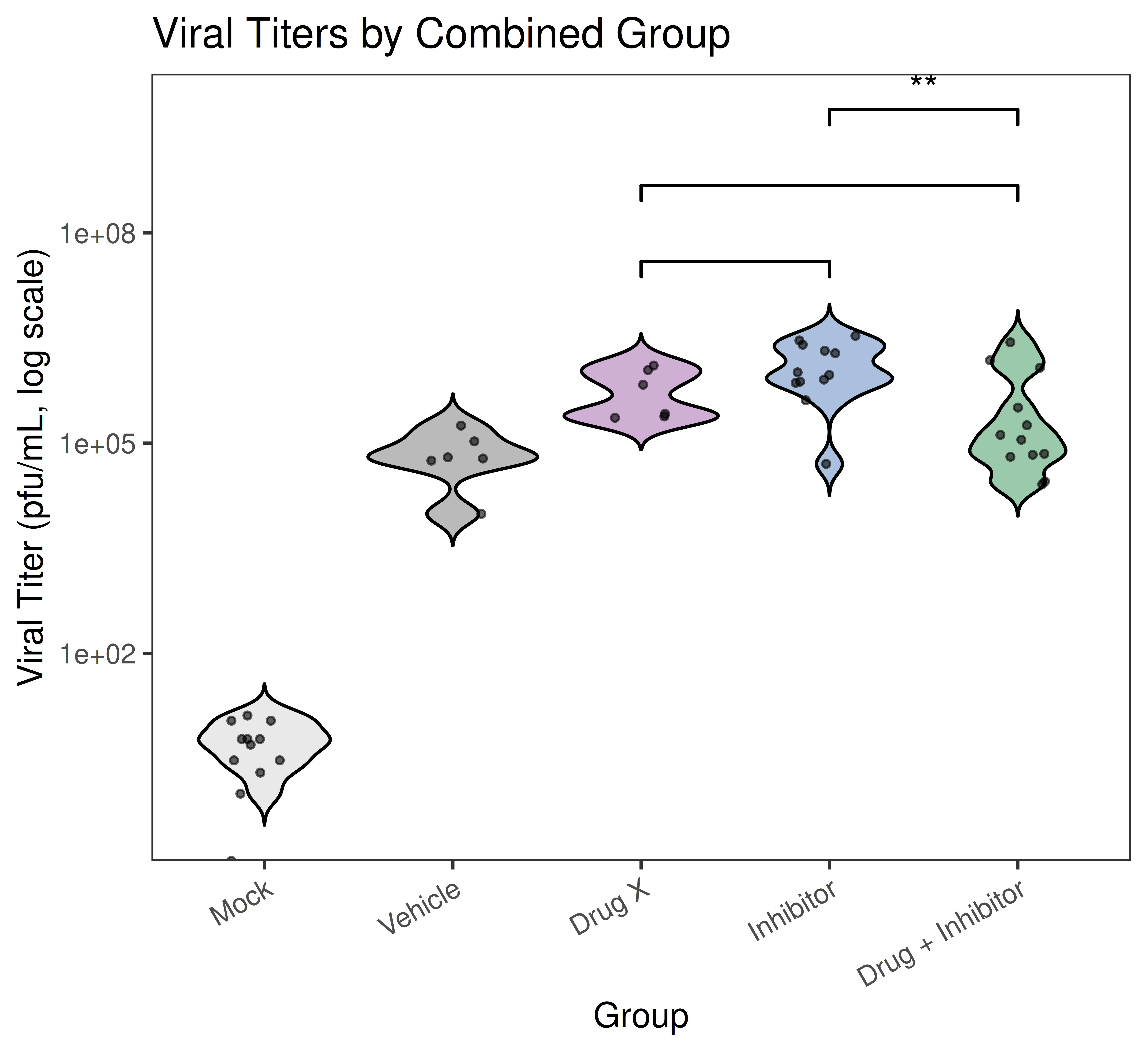
Analyzes plaque assay data from viral infection studies. Performs replicate agreement (Limits of Agreement), one-way ANOVA with Tukey HSD, and produces publication-quality violin plots on a log10 titer scale.

Overview

Item Details
Input Single CSV — one row per animal, columns for two plaque count replicates and calculated titer
Key packages ggplot2, ggpubr, rstatix, car, gt, scales
Statistics Limits of Agreement · Shapiro-Wilk · Levene · One-way ANOVA · Tukey HSD
Output Replicate QC plot · Violin plots (full + merged) · ANOVA + post-hoc tables
Download template.Rmd
Tip

When to use this template: You have viral plaque assay data with duplicate plaque counts per animal across multiple treatment groups, and you want to visualize titer distributions and test for significant differences.

Back to Gallery Open Template File

Code
## ── USER CONFIGURATION ──────────────────────────────────────────────────────
#
# DATA_FILE: Path to your CSV file with plaque assay data.
#   Expected columns (rename yours to match, or update the rename() call below):
#   - "Mouse ID"              : animal/sample identifier
#   - "Group"                 : group label (e.g., "Group 1", "Group 2")
#   - "Virus"                 : virus or mock label used in sample
#   - "# plaques counted R1"  : plaque count replicate 1
#   - "# plaques counted R2"  : plaque count replicate 2
#   - "Average plaques from duplicate wells in a 12-well plate"
#   - "Plated 10e-1 to 10e-6 dilution"
#   - "Total Volume (ml)"
#   - "pfu/mL right-side lung homogenate"  : calculated viral titer
#
DATA_FILE <- "data/titer_data.csv"

# EXCLUDE_PATTERN: Regex to drop rows you do not want (e.g., backtitrations).
#   Set to NULL to keep all rows.
EXCLUDE_PATTERN <- NULL   # e.g., "backtitration"

# GROUP_MAP: Named character vector mapping your "Group N" labels to
#   human-readable short names used in all plots and tables.
#   Keys  = values in the "Group" column of your CSV.
#   Values = display names (shown on plot axes).
GROUP_MAP <- c(
  "Group 1" = "Mock + Compound A",
  "Group 2" = "Mock + Compound B",
  "Group 3" = "Compound A",
  "Group 4" = "Compound B",
  "Group 5" = "Drug X",
  "Group 6" = "Compound A + Drug X",
  "Group 7" = "Compound B + Drug X",
  "Group 8" = "Vehicle"
)

# GROUP_ORDER: Display order on the x-axis. Must contain the same strings
#   as the values of GROUP_MAP.
GROUP_ORDER <- c(
  "Mock + Compound A",
  "Mock + Compound B",
  "Vehicle",
  "Drug X",
  "Compound A",
  "Compound A + Drug X",
  "Compound B",
  "Compound B + Drug X"
)

# PALETTE_GROUPS: Fill color for each group in the full violin plot.
#   Names must match the values of GROUP_MAP / GROUP_ORDER.
PALETTE_GROUPS <- c(
  "Mock + Compound A"    = "grey85",
  "Mock + Compound B"    = "grey70",
  "Vehicle"              = "grey40",
  "Drug X"               = "#984ea3",
  "Compound A"           = "#74add1",
  "Compound B"           = "#4575b4",
  "Compound A + Drug X"  = "#66c2a5",
  "Compound B + Drug X"  = "#238b45"
)

# MERGE_MAP: Optionally collapse related groups for the combined-group plot.
#   Keys = ShortGroup values; Values = merged display name.
#   Groups not listed here are kept as-is.
MERGE_MAP <- c(
  "Mock + Compound A"    = "Mock",
  "Mock + Compound B"    = "Mock",
  "Compound A"           = "Inhibitor",
  "Compound B"           = "Inhibitor",
  "Compound A + Drug X"  = "Drug + Inhibitor",
  "Compound B + Drug X"  = "Drug + Inhibitor",
  "Vehicle"              = "Vehicle",
  "Drug X"               = "Drug X"
)

# MERGE_ORDER: Display order for the combined-group violin plot.
MERGE_ORDER <- c("Mock", "Vehicle", "Drug X", "Inhibitor", "Drug + Inhibitor")

# PALETTE_MERGED: Fill colors for the combined-group violin plot.
PALETTE_MERGED <- c(
  "Mock"            = "grey80",
  "Vehicle"         = "grey40",
  "Drug X"          = "#984ea3",
  "Inhibitor"       = "#4575b4",
  "Drug + Inhibitor"= "#238b45"
)

# COMPARISONS: Pairs of merged groups to test with stat_compare_means().
#   Each element is a length-2 character vector of MERGE_ORDER values.
COMPARISONS <- list(
  c("Drug X", "Inhibitor"),
  c("Drug X", "Drug + Inhibitor"),
  c("Inhibitor", "Drug + Inhibitor")
)

# TITER_COL: Column name in your CSV that holds the computed titer value.
TITER_COL <- "pfu/mL right-side lung homogenate"

## ────────────────────────────────────────────────────────────────────────────

Setup

Libraries

Code
library(readr)
library(dplyr)
library(janitor)
library(stringr)
library(ggplot2)
library(scales)
library(rstatix)
library(car)
library(ggpubr)
library(gt)
library(broom)

Load Data

Code
df <- read_csv(DATA_FILE)

Clean and Organize

Code
df_clean <- df %>%
  { if (!is.null(EXCLUDE_PATTERN)) filter(., !str_detect(Group, EXCLUDE_PATTERN)) else . } %>%
  rename(
    MouseID    = `Mouse ID`,
    Plaques_R1 = `# plaques counted R1`,
    Plaques_R2 = `# plaques counted R2`,
    AvgPlaques = `Average plaques from duplicate wells in a 12-well plate`,
    Dilution   = `Plated 10e-1 to 10e-6 dilution`,
    Volume_mL  = `Total Volume (ml)`,
    Titer      = all_of(TITER_COL)
  ) %>%
  mutate(
    ShortGroup  = coalesce(unname(GROUP_MAP[Group]), Group),
    MergedGroup = coalesce(unname(MERGE_MAP[ShortGroup]), ShortGroup),
    ShortGroup  = factor(ShortGroup, levels = GROUP_ORDER),
    MergedGroup = factor(MergedGroup, levels = MERGE_ORDER),
    mean_plaques  = (Plaques_R1 + Plaques_R2) / 2,
    diff_plaques  = Plaques_R1 - Plaques_R2,
    Titer_pseudo  = Titer + 1,
    logTiter      = log10(Titer + 1)
  )

# ── Limit of Agreement (LoA) ─────────────────────────────────────────────────
loa_stats <- df_clean %>%
  summarise(
    bias    = mean(diff_plaques, na.rm = TRUE),
    sd_diff = sd(diff_plaques, na.rm = TRUE)
  )
loa_upper <- loa_stats$bias + 1.96 * loa_stats$sd_diff
loa_lower <- loa_stats$bias - 1.96 * loa_stats$sd_diff

df_clean <- df_clean %>%
  mutate(
    flag_bad_replicate = diff_plaques < loa_lower | diff_plaques > loa_upper
  )

Check Replicates

Code
labeled_points <- filter(df_clean, flag_bad_replicate)

print(
  ggplot(df_clean, aes(x = Plaques_R1, y = Plaques_R2, color = flag_bad_replicate)) +
    geom_point(size = 2) +
    geom_abline(slope = 1, intercept = 0, color = "grey40") +
    geom_text(
      data    = labeled_points,
      mapping = aes(
        x = Plaques_R1,
        y = Plaques_R2,
        label = as.character(MouseID)
      ),
      nudge_y = 1, size = 3, color = "orange", inherit.aes = FALSE
    ) +
    scale_color_manual(values = c("black", "orange"), labels = c("OK", "Outside LoA")) +
    labs(
      x     = "Plaques counted (Replicate 1)",
      y     = "Plaques counted (Replicate 2)",
      color = "Flagged",
      title = "Replicate Agreement (1.96 × SD Limits of Agreement)"
    ) +
    theme_bw() +
    theme(
      panel.grid.major = element_blank(),
      panel.grid.minor = element_blank()
    )
)

Data points outside the LoA are flagged in orange. Review these samples before proceeding.

Plots

Full Group Violin Plot

Code
p_full <- ggplot(df_clean, aes(x = ShortGroup, y = Titer, fill = ShortGroup)) +
  geom_violin(trim = FALSE, alpha = 0.7, color = "black", bw = 0.15) +
  stat_summary(
    fun.data = mean_sdl,
    fun.args = list(mult = 1),
    geom = "pointrange", color = "black", size = 0.8, alpha = 0.9, shape = 22
  ) +
  geom_jitter(width = 0.18, size = 1, alpha = 0.60) +
  scale_fill_manual(values = PALETTE_GROUPS, guide = "none") +
  scale_y_log10(labels = scales::label_scientific()) +
  labs(
    x       = "Group",
    y       = "Viral Titer (pfu/mL, log scale)",
    title   = "Viral Titers by Group",
    caption = "Black bars indicate mean \u00b1 1 SD"
  ) +
  theme_bw(base_size = 13) +
  theme(
    axis.text.x      = element_text(angle = 30, hjust = 1),
    panel.grid.major = element_blank(),
    panel.grid.minor = element_blank()
  )

ggsave("Viral_Titer_By_Group.tiff", plot = p_full,
       width = 8, height = 5, units = "in", dpi = 600,
       compression = "lzw")
print(p_full)

Combined Group Violin Plot

Code
p_merged <- ggplot(df_clean, aes(x = MergedGroup, y = Titer, fill = MergedGroup)) +
  geom_violin(trim = FALSE, alpha = 0.45, color = "black", bw = 0.15) +
  geom_jitter(width = 0.18, size = 1, alpha = 0.60) +
  scale_fill_manual(values = PALETTE_MERGED, guide = "none") +
  scale_y_log10(labels = scales::label_scientific()) +
  labs(
    x     = "Group",
    y     = "Viral Titer (pfu/mL, log scale)",
    title = "Viral Titers by Combined Group"
  ) +
  theme_bw(base_size = 13) +
  theme(
    axis.text.x      = element_text(angle = 30, hjust = 1),
    panel.grid.major = element_blank(),
    panel.grid.minor = element_blank()
  )

ggsave("Viral_Titer_By_MergedGroup.tiff", plot = p_merged,
       width = 8, height = 5, units = "in", dpi = 600,
       compression = "lzw")
print(p_merged)

Significance Testing

Assumption Checks

Code
df_clean %>%
  group_by(ShortGroup) %>%
  filter(sd(logTiter, na.rm = TRUE) > 0) %>%
  shapiro_test(logTiter)
# A tibble: 8 × 4
  ShortGroup          variable statistic      p
  <fct>               <chr>        <dbl>  <dbl>
1 Mock + Compound A   logTiter     0.936 0.630 
2 Mock + Compound B   logTiter     0.956 0.787 
3 Vehicle             logTiter     0.872 0.233 
4 Drug X              logTiter     0.827 0.100 
5 Compound A          logTiter     0.819 0.0866
6 Compound A + Drug X logTiter     0.917 0.482 
7 Compound B          logTiter     0.905 0.402 
8 Compound B + Drug X logTiter     0.884 0.286 
Code
leveneTest(logTiter ~ ShortGroup, data = df_clean)
Levene's Test for Homogeneity of Variance (center = median)
      Df F value Pr(>F)
group  7  0.9812 0.4583
      40               

One-Way ANOVA — All Groups

Code
fit_full <- aov(logTiter ~ ShortGroup, data = df_clean)

tidy(fit_full) %>%
  gt() %>%
  tab_header(title = "ANOVA: log\u2081\u2080(Titer) by Group") %>%
  fmt_number(columns = c(statistic, p.value), decimals = 3) %>%
  cols_label(term = "Source", df = "df", sumsq = "Sum Sq",
             meansq = "Mean Sq", statistic = "F value", p.value = "Pr(>F)")
ANOVA: log₁₀(Titer) by Group
Source df Sum Sq Mean Sq F value Pr(>F)
ShortGroup 7 215.730994 30.8187134 177.433 0.000
Residuals 40 6.947686 0.1736921 NA NA
Code
tukey_raw <- TukeyHSD(fit_full, conf.level = 0.95)$ShortGroup
tukey_tbl <- as.data.frame(tukey_raw)
tukey_tbl$comparison <- rownames(tukey_tbl)
rownames(tukey_tbl) <- NULL
tukey_tbl <- tukey_tbl[, c("comparison", "diff", "lwr", "upr", "p adj")]
names(tukey_tbl)[5] <- "p_adj"

tukey_tbl %>%
  gt() %>%
  tab_header(title = "Tukey HSD: Pairwise Comparisons") %>%
  fmt_number(columns = c(diff, lwr, upr, p_adj), decimals = 3) %>%
  cols_label(comparison = "Comparison", diff = "Difference",
             lwr = "Lower CI", upr = "Upper CI", p_adj = "Adjusted p")
Tukey HSD: Pairwise Comparisons
Comparison Difference Lower CI Upper CI Adjusted p
Mock + Compound B-Mock + Compound A −0.173 −0.942 0.596 0.996
Vehicle-Mock + Compound A 3.963 3.194 4.732 0.000
Drug X-Mock + Compound A 4.888 4.119 5.658 0.000
Compound A-Mock + Compound A 5.329 4.560 6.098 0.000
Compound A + Drug X-Mock + Compound A 4.959 4.190 5.728 0.000
Compound B-Mock + Compound A 5.054 4.285 5.823 0.000
Compound B + Drug X-Mock + Compound A 3.930 3.161 4.699 0.000
Vehicle-Mock + Compound B 4.136 3.367 4.905 0.000
Drug X-Mock + Compound B 5.061 4.292 5.830 0.000
Compound A-Mock + Compound B 5.502 4.732 6.271 0.000
Compound A + Drug X-Mock + Compound B 5.132 4.363 5.901 0.000
Compound B-Mock + Compound B 5.227 4.458 5.996 0.000
Compound B + Drug X-Mock + Compound B 4.103 3.334 4.872 0.000
Drug X-Vehicle 0.925 0.156 1.694 0.009
Compound A-Vehicle 1.366 0.596 2.135 0.000
Compound A + Drug X-Vehicle 0.996 0.227 1.765 0.004
Compound B-Vehicle 1.091 0.322 1.860 0.001
Compound B + Drug X-Vehicle −0.033 −0.802 0.736 1.000
Compound A-Drug X 0.440 −0.329 1.209 0.604
Compound A + Drug X-Drug X 0.071 −0.698 0.840 1.000
Compound B-Drug X 0.166 −0.604 0.935 0.997
Compound B + Drug X-Drug X −0.958 −1.728 −0.189 0.006
Compound A + Drug X-Compound A −0.369 −1.139 0.400 0.784
Compound B-Compound A −0.275 −1.044 0.494 0.943
Compound B + Drug X-Compound A −1.399 −2.168 −0.630 0.000
Compound B-Compound A + Drug X 0.095 −0.675 0.864 1.000
Compound B + Drug X-Compound A + Drug X −1.029 −1.798 −0.260 0.003
Compound B + Drug X-Compound B −1.124 −1.893 −0.355 0.001

One-Way ANOVA — Combined Groups

Code
fit_merged <- aov(logTiter ~ MergedGroup, data = df_clean)

tidy(fit_merged) %>%
  gt() %>%
  tab_header(title = "ANOVA: log\u2081\u2080(Titer) by Merged Group") %>%
  fmt_number(columns = c(statistic, p.value), decimals = 3) %>%
  cols_label(term = "Source", df = "df", sumsq = "Sum Sq",
             meansq = "Mean Sq", statistic = "F value", p.value = "Pr(>F)")
ANOVA: log₁₀(Titer) by Merged Group
Source df Sum Sq Mean Sq F value Pr(>F)
MergedGroup 4 212.23629 53.0590719 218.488 0.000
Residuals 43 10.44239 0.2428463 NA NA
Code
tukey_m_raw <- TukeyHSD(fit_merged, conf.level = 0.95)$MergedGroup
tukey_m_tbl <- as.data.frame(tukey_m_raw)
tukey_m_tbl$comparison <- rownames(tukey_m_tbl)
rownames(tukey_m_tbl) <- NULL
tukey_m_tbl <- tukey_m_tbl[, c("comparison", "diff", "lwr", "upr", "p adj")]
names(tukey_m_tbl)[5] <- "p_adj"

tukey_m_tbl %>%
  gt() %>%
  tab_header(title = "Tukey HSD: Merged Group Pairwise Comparisons") %>%
  fmt_number(columns = c(diff, lwr, upr, p_adj), decimals = 3) %>%
  cols_label(comparison = "Comparison", diff = "Difference",
             lwr = "Lower CI", upr = "Upper CI", p_adj = "Adjusted p")
Tukey HSD: Merged Group Pairwise Comparisons
Comparison Difference Lower CI Upper CI Adjusted p
Vehicle-Mock 4.050 3.348 4.751 0.000
Drug X-Mock 4.975 4.273 5.676 0.000
Inhibitor-Mock 5.278 4.705 5.851 0.000
Drug + Inhibitor-Mock 4.531 3.958 5.104 0.000
Drug X-Vehicle 0.925 0.115 1.735 0.018
Inhibitor-Vehicle 1.228 0.527 1.930 0.000
Drug + Inhibitor-Vehicle 0.481 −0.220 1.183 0.305
Inhibitor-Drug X 0.303 −0.399 1.004 0.734
Drug + Inhibitor-Drug X −0.444 −1.145 0.258 0.386
Drug + Inhibitor-Inhibitor −0.747 −1.319 −0.174 0.005

Violin Plot with Significance Brackets

Code
df_plot <- df_clean %>% filter(!is.na(Titer) & Titer >= 0)

p_combined <- ggplot(df_plot, aes(x = MergedGroup, y = Titer, fill = MergedGroup)) +
  geom_violin(trim = FALSE, alpha = 0.45, color = "black", bw = 0.15) +
  geom_jitter(width = 0.18, size = 1, alpha = 0.60) +
  scale_fill_manual(values = PALETTE_MERGED, guide = "none") +
  scale_y_log10(labels = scales::label_scientific()) +
  expand_limits(y = max(df_plot$Titer, na.rm = TRUE) * 5) +
  labs(
    x     = "Group",
    y     = "Viral Titer (pfu/mL, log scale)",
    title = "Viral Titers by Combined Group"
  ) +
  theme_bw(base_size = 13) +
  theme(
    axis.text.x      = element_text(angle = 30, hjust = 1),
    panel.grid.major = element_blank(),
    panel.grid.minor = element_blank()
  ) +
  stat_compare_means(
    comparisons  = COMPARISONS,
    method       = "t.test",
    label        = "p.signif",
    hide.ns      = TRUE,
    size         = 5,
    bracket.size = 0.6,
    step.increase = 0.15
  )

ggsave("Viral_Titer_CombinedGroups_sig.tiff", plot = p_combined,
       width = 8, height = 5.5, units = "in", dpi = 600,
       compression = "lzw")
print(p_combined)