---
title: "11 · Variant Frequency + Shannon Entropy"
subtitle: "Intra-host variant frequency scatter, Shannon entropy curves, and caller-overlap Venn diagrams"
description: |
LoFreq and iVar variant calls across days post-infection (DPI). Variant frequency
scatter plots with gene-boundary annotation, genome-wide Shannon entropy trajectories
with SEM ribbons, and caller-overlap Venn diagrams to quantify agreement.
categories: [genomics, virology, variant-calling, entropy, Shannon, LoFreq, iVar]
jupyter: python3
---
## Overview
| Item | Details |
|------|---------|
| **Input** | CSV variant tables: `LoFreq_variants.csv`, `iVar_variants.csv`, `gene_coords.csv`, `manifest.csv` |
| **Key packages** | `pandas`, `numpy`, `matplotlib`, `scipy`, `matplotlib_venn` (optional) |
| **Statistics** | Shannon entropy (natural log) · Allele frequency filtering · Caller overlap |
| **Output** | Variant frequency scatter (SVG/PNG) · Entropy curves (SVG/PNG) · Venn diagram (SVG/PNG) |
| **Download** | [template.qmd](template.qmd) |
Edit `FILTER_MIN_DP` and `FILTER_MIN_AF` to set depth and allele-frequency cut-offs. Modify `DPI_CONFIG` to control colour and display order for each DPI group. Set `GENOME_LENGTH` to your reference length — it is *not* inferred from the gene annotation, which would silently drop any variant past the last annotated gene.
[← Gallery](../../index.html){.btn .btn-outline-secondary}
[Download .qmd](template.qmd){.btn .btn-primary}
---
## User Configuration
```{python}
#| label: user-config
# ── USER CONFIGURATION ────────────────────────────────────────────────────────

# Minimum read depth to retain a variant
FILTER_MIN_DP = 500

# Minimum allele frequency to retain a variant (e.g. 0.01 = 1%)
FILTER_MIN_AF = 0.01

# Paths to input data (relative to this file)
LOFREQ_CSV   = "data/LoFreq_variants.csv"
IVAR_CSV     = "data/iVar_variants.csv"
GENE_COORDS  = "data/gene_coords.csv"
MANIFEST_CSV = "data/manifest.csv"

# DPI group configuration — colours must match Okabe-Ito palette
DPI_CONFIG = {
    1: {"label": "DPI 1", "color": "#E69F00"},
    3: {"label": "DPI 3", "color": "#56B4E9"},
    5: {"label": "DPI 5", "color": "#009E73"},
}

# Reference genome length (nt). Set this explicitly — deriving it from the gene
# annotation drops every variant downstream of the last annotated gene.
GENOME_LENGTH = 11447

# Output directory for plots
OUTPUT_DIR = "outputs"

# Sliding-window size for entropy curves (genomic positions).
# Pick this against your variant density, not for its own sake: the window has to hold
# enough variants for the windowed sum to mean anything. At ~115 variants per sample over
# an 11.4 kb genome, a 200 nt window holds ~2 variants and the curve is pure noise; 1000 nt
# holds ~10 and the regional structure becomes visible.
WINDOW_SIZE = 1000

# Step between successive entropy windows (nt). Smaller is smoother and slower; anything
# well below WINDOW_SIZE gives a continuous-looking curve.
WINDOW_STEP = 25

# ─────────────────────────────────────────────────────────────────────────────
```
## Setup
```{python}
#| label: setup
import os
import warnings

import numpy as np
import pandas as pd
import matplotlib.pyplot as plt

# Narrow suppression only: numpy raises this when a sliding window happens to hold
# a single variant, where the sample standard deviation is undefined by design.
warnings.filterwarnings("ignore", category=RuntimeWarning,
                        message="Degrees of freedom <= 0")

# ── Global plot theme: white background, no grid, black spine, Arial ─────────
# Reproducible SVG output: matplotlib stamps a wall-clock date and randomly
# generated element IDs into every SVG, so re-rendering an unchanged figure
# produced a large but meaningless git diff. A fixed salt and a fixed
# SOURCE_DATE_EPOCH make repeat renders byte-identical.
os.environ.setdefault("SOURCE_DATE_EPOCH", "1735689600")   # 2025-01-01 UTC
plt.rcParams["svg.hashsalt"] = "lab-bioinfo-templates"

plt.rcParams.update({
    "font.family":      "sans-serif",
    "font.sans-serif":  ["Arial", "Helvetica", "DejaVu Sans"],
    "axes.facecolor":   "white",
    "figure.facecolor": "white",
    "axes.grid":        False,
    "axes.edgecolor":   "black",
    "axes.linewidth":   1.0,
    "axes.spines.top":    True,
    "axes.spines.right": True,
    "axes.titlesize":    12,
    "axes.labelsize":    10,
    "xtick.labelsize":   9,
    "ytick.labelsize":   9,
    "legend.fontsize":   9,
    "figure.dpi":       150,
})
pd.set_option("display.width", 1000)

os.makedirs(OUTPUT_DIR, exist_ok=True)
print(f"Output will be saved to: {os.path.abspath(OUTPUT_DIR)}")

# ── Okabe-Ito palette helpers ────────────────────────────────────────────────
OKABE_ITO = {
    "orange":       "#E69F00",
    "sky_blue":     "#56B4E9",
    "bluish_green": "#009E73",
    "amber":        "#F5C710",
    "blue":         "#0072B2",
    "vermillion":   "#D55E00",
    "reddish_purple": "#CC79A7",
    "black":        "#000000",
}

DPI_COLORS = {dpi: cfg["color"] for dpi, cfg in DPI_CONFIG.items()}
DPI_LABELS = {dpi: cfg["label"] for dpi, cfg in DPI_CONFIG.items()}
DPI_ORDER  = sorted(DPI_CONFIG.keys())
```
## Load Data
```{python}
#| label: load-data
def require_columns(df, required, name):
    """Fail loudly if an input table is missing a column the analysis depends on."""
    missing = set(required) - set(df.columns)
    if missing:
        raise ValueError(
            f"{name} is missing required column(s): {sorted(missing)}. "
            f"Found: {list(df.columns)}"
        )

manifest = pd.read_csv(MANIFEST_CSV)
require_columns(manifest, ["sample_id", "dpi"], MANIFEST_CSV)
print(f"Manifest: {len(manifest)} samples")
print(manifest.head(), "\n")

gene_coords = pd.read_csv(GENE_COORDS)
require_columns(gene_coords, ["gene", "start", "end"], GENE_COORDS)
print(f"Gene coordinates: {len(gene_coords)} genes")
print(gene_coords.head(), "\n")

lofreq_raw = pd.read_csv(LOFREQ_CSV)
ivar_raw   = pd.read_csv(IVAR_CSV)
print(f"LoFreq: {len(lofreq_raw)} variants")
print(f"iVar:   {len(ivar_raw)} variants")

for df, name in [(lofreq_raw, LOFREQ_CSV), (ivar_raw, IVAR_CSV)]:
    require_columns(df, ["AF", "DP", "POS", "sample_id", "dpi"], name)

# Merge variant data into a single DataFrame with a 'caller' column
lofreq_raw["caller"] = "LoFreq"
ivar_raw["caller"]   = "iVar"
all_vars = pd.concat([lofreq_raw, ivar_raw], ignore_index=True)

CALLERS = ["LoFreq", "iVar"]

# Cross-check the per-variant DPI against the manifest: a sample_id whose dpi
# disagrees with its manifest row would scatter that variant into the wrong group.
dpi_map = dict(zip(manifest["sample_id"], manifest["dpi"]))
expected_dpi = all_vars["sample_id"].map(dpi_map)
unknown = sorted(all_vars.loc[expected_dpi.isna(), "sample_id"].unique())
if unknown:
    raise ValueError(f"sample_id(s) absent from {MANIFEST_CSV}: {unknown}")
mismatch = all_vars.loc[expected_dpi != all_vars["dpi"]]
if len(mismatch):
    raise ValueError(
        f"{len(mismatch)} variant row(s) have a 'dpi' that disagrees with "
        f"{MANIFEST_CSV}, e.g.\n{mismatch.head()[['sample_id', 'dpi', 'caller']]}"
    )

# Positions outside the reference are a data error, not something to drop quietly.
off_genome = all_vars[(all_vars["POS"] < 1) | (all_vars["POS"] > GENOME_LENGTH)]
if len(off_genome):
    raise ValueError(
        f"{len(off_genome)} variant(s) fall outside GENOME_LENGTH={GENOME_LENGTH} "
        f"(positions {off_genome['POS'].min()}–{off_genome['POS'].max()}). "
        f"Check GENOME_LENGTH against your reference."
    )

print(f"\nCombined: {len(all_vars)} total variants")
all_vars.head()
```
## Quality Control: Depth & Frequency Filtering
```{python}
#| label: qc-filter
pre = len(all_vars)
all_vars = all_vars[
    (all_vars["DP"] >= FILTER_MIN_DP) &
    (all_vars["AF"] >= FILTER_MIN_AF)
].copy()
print(f"Retained {len(all_vars)} / {pre} variants "
      f"(DP ≥ {FILTER_MIN_DP}, AF ≥ {FILTER_MIN_AF})")

# Assign variant classification for plotting.
# Gene first: an intergenic position has no reading frame, so any coding
# consequence attached to it is meaningless and must not win the classification.
def classify_variant(row):
    if row.get("gene", "") == "intergenic":
        return "intergenic"
    elif row.get("consequence", "") == "missense_variant":
        return "missense"
    else:
        return "synonymous/other"

all_vars["variant_class"] = all_vars.apply(classify_variant, axis=1)
print(all_vars["variant_class"].value_counts().to_string())
```
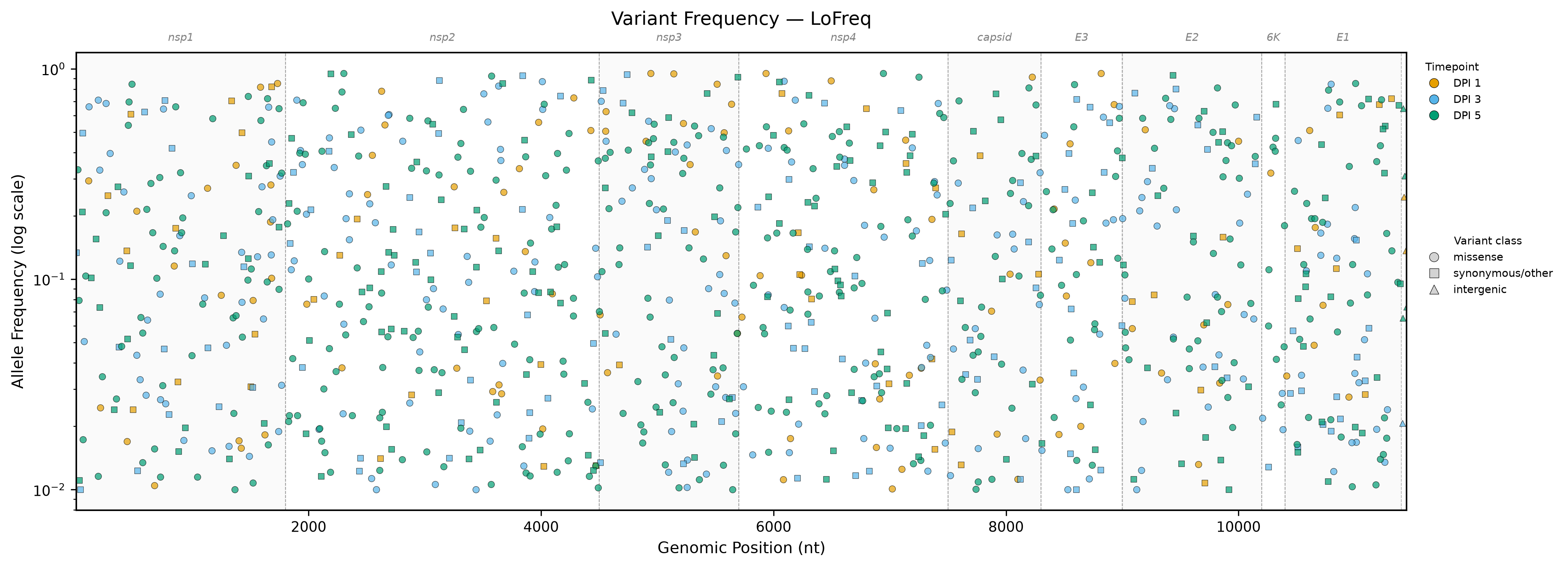
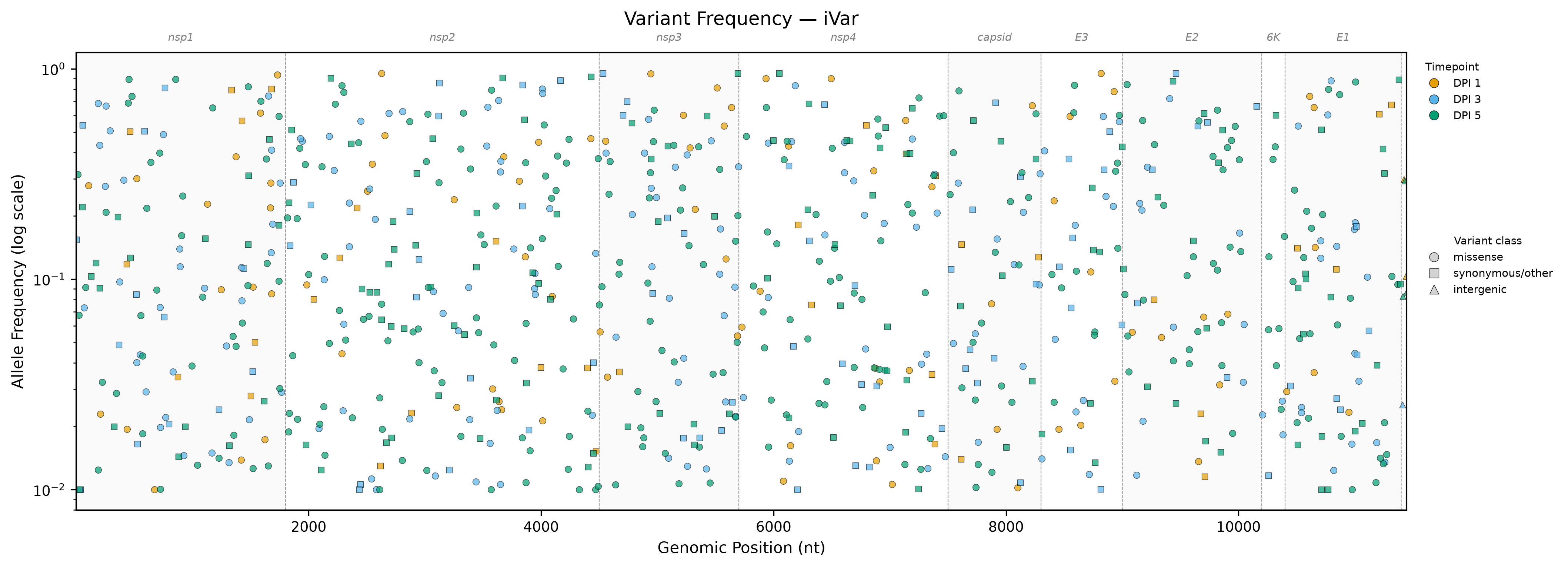
## 1. Variant Frequency Scatter
Genomic position on the x-axis, log10(allele frequency) on the y-axis, with gene
boundaries as vertical spans and DPI as colour.
```{python}
#| label: plot-variant-scatter
#| fig-width: 14
#| fig-height: 5
# Define marker shapes per variant class
class_styles = {
    "missense":       {"marker": "o", "s": 18, "edgecolors": "black", "linewidths": 0.3},
    "synonymous/other": {"marker": "s", "s": 14, "edgecolors": "black", "linewidths": 0.3},
    "intergenic":     {"marker": "^", "s": 16, "edgecolors": "black", "linewidths": 0.3},
}

from matplotlib.lines import Line2D

for caller in CALLERS:
    fig, ax = plt.subplots(figsize=(14, 5), constrained_layout=True)
    cdf = all_vars[all_vars["caller"] == caller]

    for dpi in DPI_ORDER:
        sub = cdf[cdf["dpi"] == dpi]
        for vclass, style in class_styles.items():
            pts = sub[sub["variant_class"] == vclass]
            if pts.empty:
                continue
            ax.scatter(
                pts["POS"], pts["AF"],
                c=DPI_COLORS[dpi],
                marker=style["marker"],
                s=style["s"],
                edgecolors=style["edgecolors"],
                linewidths=style["linewidths"],
                alpha=0.7,
                zorder=2,
            )

    # Gene annotation: alternating grey bands with the names above the axis, matching
    # templates 11's entropy panel and 12. Colour is reserved for DPI here.
    for i, (_, gene_row) in enumerate(gene_coords.iterrows()):
        if i % 2 == 0:
            ax.axvspan(gene_row["start"], gene_row["end"],
                       alpha=0.04, color="grey", zorder=0)
        ax.axvline(gene_row["start"], color="grey", linestyle="--",
                   linewidth=0.5, alpha=0.5, zorder=0)
        ax.axvline(gene_row["end"], color="grey", linestyle="--",
                   linewidth=0.5, alpha=0.5, zorder=0)
        ax.annotate(
            gene_row["gene"],
            xy=((gene_row["start"] + gene_row["end"]) / 2, 1.02),
            xycoords=("data", "axes fraction"),
            ha="center", va="bottom", fontsize=7,
            fontstyle="italic", color="grey",
        )

    ax.set_yscale("log")
    ax.set_ylabel("Allele Frequency (log scale)")
    ax.set_xlabel("Genomic Position (nt)")
    ax.set_title(f"Variant Frequency — {caller}", pad=18)  # clear the gene labels
    ax.set_xlim(1, GENOME_LENGTH)

    # Two legends, because the plot encodes two independent things: colour is the
    # timepoint and marker is the variant class. Labelling only the first DPI (as this
    # did before) left the other DPIs' colours unexplained. Both sit outside the axes
    # so they cannot cover data points.
    dpi_handles = [
        Line2D([], [], linestyle="none", marker="o", markersize=6,
               markerfacecolor=DPI_COLORS[d], markeredgecolor="black",
               markeredgewidth=0.3, label=DPI_LABELS[d])
        for d in DPI_ORDER
    ]
    class_handles = [
        Line2D([], [], linestyle="none", marker=style["marker"], markersize=6,
               markerfacecolor="lightgrey", markeredgecolor="black",
               markeredgewidth=0.3, label=vclass)
        for vclass, style in class_styles.items()
    ]

    leg1 = ax.legend(handles=dpi_handles, title="Timepoint", fontsize=7,
                     title_fontsize=7, frameon=False, loc="upper left",
                     bbox_to_anchor=(1.005, 1.0))
    ax.add_artist(leg1)
    ax.legend(handles=class_handles, title="Variant class", fontsize=7,
              title_fontsize=7, frameon=False, loc="upper left",
              bbox_to_anchor=(1.005, 0.62))

    out_svg = os.path.join(OUTPUT_DIR, f"variant_scatter_{caller}.svg")
    out_png = os.path.join(OUTPUT_DIR, f"variant_scatter_{caller}.png")
    fig.savefig(out_svg, format="svg", bbox_inches="tight")
    fig.savefig(out_png, format="png", bbox_inches="tight", dpi=150)
    plt.show()
    print(f"Saved: {out_svg}, {out_png}")
```
## 2. Shannon Entropy Curves per DPI
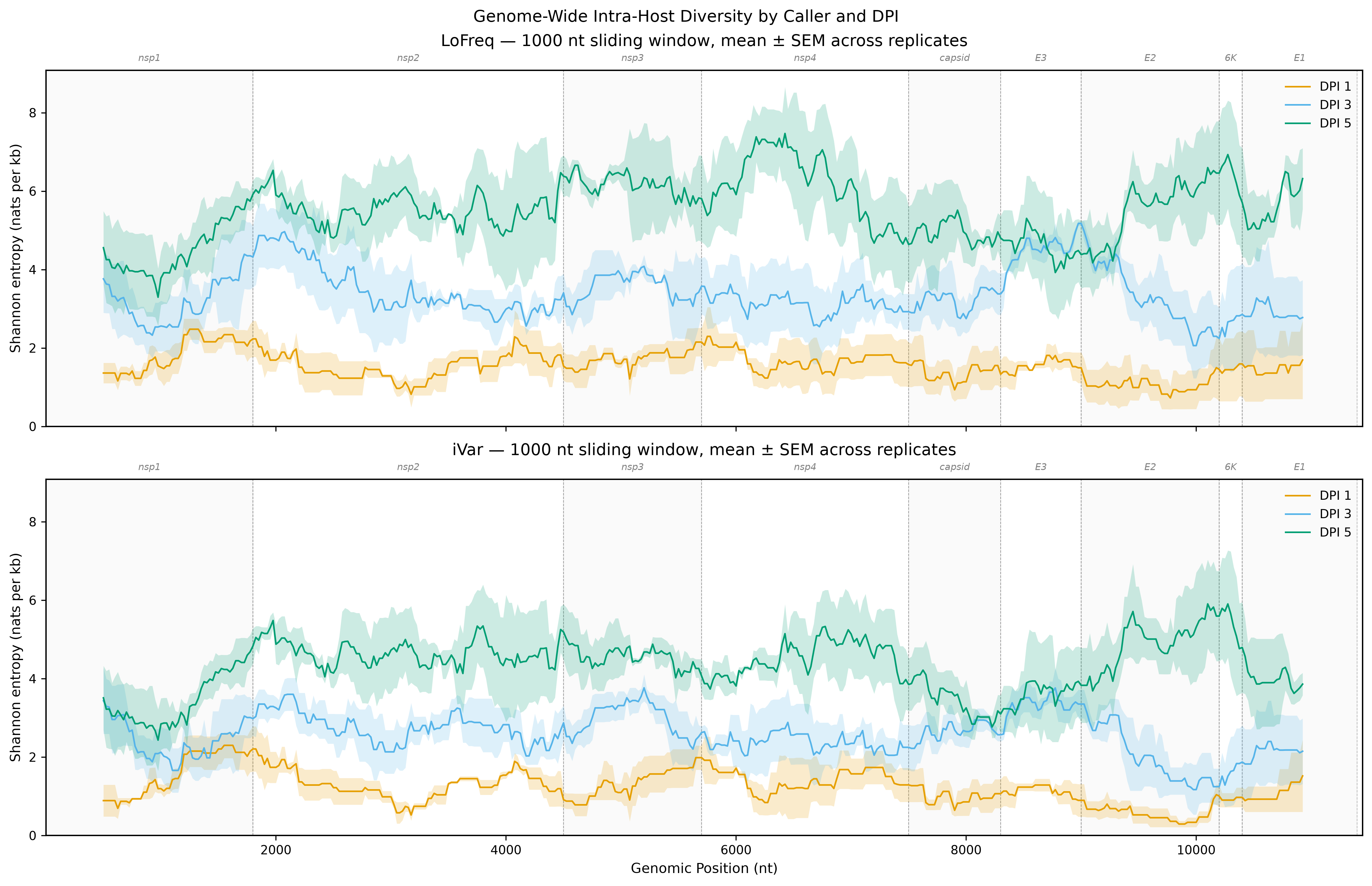
Sliding-window Shannon entropy computed genome-wide. A separate curve (mean ± SEM)
is drawn for each DPI group so that entropy accumulation can be compared through the
course of infection.
**One panel per caller.** A variant found by both callers appears once in each panel,
never twice in the same curve — pooling the callers would double-weight exactly the
concordant variants and leave the discordant ones under-weighted.
```{python}
#| label: entropy-curves
#| fig-width: 14
#| fig-height: 9
SEM_ALPHA = 0.20

def shannon_entropy(af_values):
    """Binary Shannon entropy (natural log) for a list of variant AFs. Expects AFs as float."""
    vals = np.asarray(af_values, dtype=float)
    ref_freq = 1.0 - vals
    return -(vals * np.log(vals + 1e-300) + ref_freq * np.log(ref_freq + 1e-300))


def windowed_entropy_density(frame):
    """Windowed Shannon-entropy density for ONE sample, in nats per kb.

    Each window is scored by the SUM of its variants' entropies, normalised to a
    per-kb rate. Summing (rather than averaging) is what makes this track intra-host
    diversity: a timepoint that carries more polymorphic sites scores higher, whereas a
    mean over variants is roughly flat no matter how many there are.

    A window with no variants scores 0 — genuinely zero diversity, not missing data — so
    the curve stays continuous instead of being interpolated across dropped windows.
    """
    ent_sum = np.zeros(GENOME_LENGTH + 1)   # 1-based, index 0 unused

    pos = frame["POS"].to_numpy(dtype=int)
    ent = shannon_entropy(frame["AF"].to_numpy(dtype=float))
    np.add.at(ent_sum, pos, ent)

    c_sum = np.concatenate([[0.0], np.cumsum(ent_sum)])

    starts = np.arange(1, GENOME_LENGTH - WINDOW_SIZE + 2, WINDOW_STEP)
    ends = starts + WINDOW_SIZE - 1
    total = c_sum[ends] - c_sum[starts - 1]

    centers = (starts + ends) / 2.0
    density = total * 1000.0 / WINDOW_SIZE
    return centers, density


def entropy_curve_across_replicates(frame):
    """Mean +/- SEM of the windowed entropy density ACROSS replicate samples.

    The band therefore shows between-animal spread at each position, which is the
    quantity worth seeing. (Computing a SEM across the handful of variants inside a
    single window instead says nothing and swamps the plot.)
    """
    sample_ids = sorted(frame["sample_id"].unique())
    curves = []
    centers = None
    for sid in sample_ids:
        centers, density = windowed_entropy_density(frame[frame["sample_id"] == sid])
        curves.append(density)

    if not curves:
        return np.array([]), np.array([]), np.array([])

    stacked = np.vstack(curves)
    mean = stacked.mean(axis=0)
    if stacked.shape[0] > 1:
        sem = stacked.std(axis=0, ddof=1) / np.sqrt(stacked.shape[0])
    else:
        sem = np.zeros_like(mean)
    return centers, mean, sem


# Plot: one row per caller, one curve per DPI.
fig, axes = plt.subplots(len(CALLERS), 1, figsize=(14, 4.5 * len(CALLERS)),
                         sharex=True, sharey=True, constrained_layout=True,
                         squeeze=False)
axes = axes.ravel()

for ax, caller in zip(axes, CALLERS):
    caller_vars = all_vars[all_vars["caller"] == caller]

    for dpi in DPI_ORDER:
        sub = caller_vars[caller_vars["dpi"] == dpi]
        if sub.empty:
            continue
        x_pos, y_mean, y_sem = entropy_curve_across_replicates(sub)
        if len(x_pos) == 0:
            continue
        ax.plot(x_pos, y_mean, color=DPI_COLORS[dpi], linewidth=1.2,
                label=DPI_LABELS[dpi])
        ax.fill_between(x_pos, y_mean - y_sem, y_mean + y_sem,
                        color=DPI_COLORS[dpi], alpha=SEM_ALPHA, linewidth=0)

    # Gene annotation, matching template 12: alternating grey bands plus boundary
    # rules, with the gene names above the top axis. A per-gene rainbow reads as
    # decoration and competes with the DPI colours, which carry the actual signal.
    for i, (_, gene_row) in enumerate(gene_coords.iterrows()):
        if i % 2 == 0:
            ax.axvspan(gene_row["start"], gene_row["end"],
                       alpha=0.04, color="grey", zorder=0)
        ax.axvline(gene_row["start"], color="grey", linestyle="--",
                   linewidth=0.5, alpha=0.5, zorder=0)
        ax.axvline(gene_row["end"], color="grey", linestyle="--",
                   linewidth=0.5, alpha=0.5, zorder=0)
        ax.annotate(
            gene_row["gene"],
            xy=((gene_row["start"] + gene_row["end"]) / 2, 1.02),
            xycoords=("data", "axes fraction"),
            ha="center", va="bottom", fontsize=7,
            fontstyle="italic", color="grey",
        )

    ax.set_xlim(1, GENOME_LENGTH)
    ax.set_ylabel("Shannon entropy (nats per kb)")
    ax.set_title(f"{caller} — {WINDOW_SIZE} nt sliding window, mean ± SEM across replicates",
                 pad=18)  # clear the gene labels
    ax.legend(loc="upper right", frameon=False)

axes[-1].set_xlabel("Genomic Position (nt)")
ax.set_ylim(bottom=0)
fig.suptitle("Genome-Wide Intra-Host Diversity by Caller and DPI")

out_svg = os.path.join(OUTPUT_DIR, "entropy_curves.svg")
out_png = os.path.join(OUTPUT_DIR, "entropy_curves.png")
fig.savefig(out_svg, format="svg", bbox_inches="tight")
fig.savefig(out_png, format="png", bbox_inches="tight", dpi=150)
plt.show()
print(f"Saved: {out_svg}, {out_png}")
```
## 3. LoFreq vs iVar Caller Overlap (Venn)
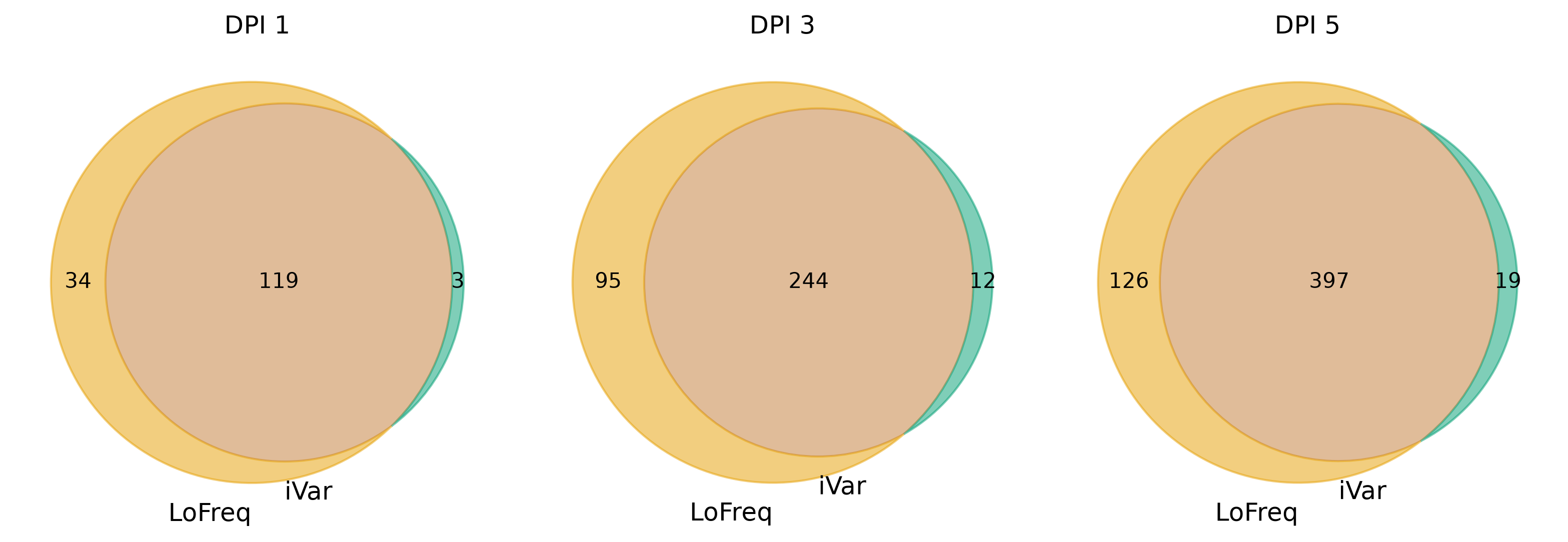
Shared variant positions between LoFreq and iVar, per DPI group. Uses
`matplotlib_venn` if installed; otherwise prints a contingency table.
```{python}
#| label: caller-venn
#| fig-width: 10
#| fig-height: 4
lofreq_positions = {
    dpi: set(all_vars[(all_vars["caller"] == "LoFreq") & (all_vars["dpi"] == dpi)]["POS"])
    for dpi in DPI_ORDER
}
ivar_positions = {
    dpi: set(all_vars[(all_vars["caller"] == "iVar") & (all_vars["dpi"] == dpi)]["POS"])
    for dpi in DPI_ORDER
}

try:
    from matplotlib_venn import venn2

    n_dpis = len(DPI_ORDER)
    fig, axes = plt.subplots(1, n_dpis, figsize=(n_dpis * 3.5, 3.5),
                             constrained_layout=True)
    if n_dpis == 1:
        axes = [axes]

    for ax, dpi in zip(axes, DPI_ORDER):
        lf_set = lofreq_positions.get(dpi, set())
        iv_set = ivar_positions.get(dpi, set())

        v = venn2(
            subsets=(len(lf_set - iv_set), len(iv_set - lf_set), len(lf_set & iv_set)),
            set_labels=("LoFreq", "iVar"),
            ax=ax,
        )
        if v.get_label_by_id("10"):
            v.get_label_by_id("10").set_text(len(lf_set - iv_set))
        if v.get_label_by_id("01"):
            v.get_label_by_id("01").set_text(len(iv_set - lf_set))
        if v.get_label_by_id("11"):
            v.get_label_by_id("11").set_text(len(lf_set & iv_set))

        # Apply Okabe-Ito colours to the diagram
        for patch_id, color in [("10", OKABE_ITO["orange"]), ("01", OKABE_ITO["bluish_green"])]:
            p = v.get_patch_by_id(patch_id)
            if p:
                p.set_color(color)
                p.set_alpha(0.5)

        ax.set_title(DPI_LABELS[dpi])

    out_svg = os.path.join(OUTPUT_DIR, "caller_overlap_venn.svg")
    out_png = os.path.join(OUTPUT_DIR, "caller_overlap_venn.png")
    fig.savefig(out_svg, format="svg", bbox_inches="tight")
    fig.savefig(out_png, format="png", bbox_inches="tight", dpi=150)
    plt.show()
    print(f"Saved: {out_svg}, {out_png}")

except ImportError:
    print(
        "matplotlib_venn is not installed — the overlap contingency table below "
        "carries the same numbers.\nInstall the figure with: pip install matplotlib-venn"
    )
```
```{python}
#| label: caller-overlap-table
# Always write the overlap numbers, whether or not matplotlib_venn drew the figure.
overlap_df = pd.DataFrame([
    {
        "DPI":          dpi,
        "LoFreq only":  len(lofreq_positions.get(dpi, set()) - ivar_positions.get(dpi, set())),
        "iVar only":    len(ivar_positions.get(dpi, set()) - lofreq_positions.get(dpi, set())),
        "Shared":       len(lofreq_positions.get(dpi, set()) & ivar_positions.get(dpi, set())),
        "Total union":  len(lofreq_positions.get(dpi, set()) | ivar_positions.get(dpi, set())),
    }
    for dpi in DPI_ORDER
])
overlap_df["Jaccard"] = (overlap_df["Shared"] / overlap_df["Total union"]).round(3)
overlap_df.to_csv(os.path.join(OUTPUT_DIR, "caller_overlap_summary.csv"), index=False)
print("Saved: caller_overlap_summary.csv")
overlap_df
```
## Summary: Variant Counts per DPI per Caller
```{python}
#| label: summary-table
summary = (
    all_vars
    .groupby(["dpi", "caller"])["POS"]
    .count()
    .unstack(fill_value=0)
)
summary.columns.name = None
summary.index.name = "DPI"

# Variant-class breakdown, kept split by caller: a variant both callers report is
# one call per caller, and collapsing the caller axis would count it twice.
class_summary = (
    all_vars
    .groupby(["caller", "dpi", "variant_class"])["POS"]
    .count()
    .unstack(fill_value=0)
)

print("=== Variants per DPI per Caller ===")
print(summary.to_string())
print("\n=== Variant classes per DPI per Caller ===")
print(class_summary.to_string())
print(f"\n{len(all_vars)} filtered variant calls in total "
      f"(each caller counted separately).")
summary.to_csv(os.path.join(OUTPUT_DIR, "variant_summary_by_caller.csv"))
class_summary.to_csv(os.path.join(OUTPUT_DIR, "variant_summary_by_class.csv"))
print("Saved: variant_summary_by_caller.csv, variant_summary_by_class.csv")
```